COS 484
Natural Language Processing
Written live in classes with Prof. Karthik Narasimhan and Prof. Tri Dao.
Last updated: 02/26.
Contents
- Introduction & Language Models
- Text Classification
- Word Embeddings
- Neural networks for NLP
- Sequence Models
- Recurrent Neural Networks
- Seq2seq Models & Attention
- Self-attention & Transformers
- Self-attention II
- Contexualized Representations and Pre-training
Lecture 1
Introduction & Language Models
Natural language processing or NLP is a rapidly-evolving field, that is becoming increasingly central to our daily lives, as chatbots become more widely integrated.
NLP is an interdisciplinary field, building computer programs to analyze, understand and generate human language - either spoken or written.
Why is language difficult to understand? It can be ambiguous; there are dialects and accents; context and dependencies matter; there could be humour, sarcasm or irony etc.
The roadmap for this course is in four parts as below:
- $N$-gram language models; text classification; word embeddings; neural ents for language.
- Sequence models; recurrent neural nets; attention; transformers.
- Large language models (pre-training, adaptation, post-training); language agents.
- Systems for LLMs; evaluations and data; reasoning.
Language models
A language model is a probabilisitc model of a sequence of words.
The joint probability distribution of words $w_1,w_2,\dots,w_n$ is $P(w_1,w_2,\dots,w_n)$, i.e. how likely is a given phrase, sentence, paragraph or even document.
To make computations easier, we have the chain rule for probabilties, by conditioning on previous words.
\[P(w_1,\dots,w_n) = P(w_1)P(w_2\mid w_1)P(w_3\mid w_2,w_1)\times\dots\times P(w_n\mid w_1,\dots,w_{n-1})\]Language models are everywhere - a common example being in auto-complete on your phone, or auto-completion of query suggestions in search engine.
For estimating probabilities, we can use the simple MLE of
\[P(w_3 \mid w_1,w_2) = \frac{\text{count}(w_1 w_2 w_3)}{\text{count}(w_1w_2)}.\]It is common to introduce a Markov assumption, which means using only the recent past to predict the next word, in order to simplify computations.
This reduces the number of estimated parameters in exchange for modelling capacity.
For instance, the $k$-th order Markov assumption considers only the last $k$ words (or less) when conditioning.
\[\therefore \hspace{5pt} P(w_i\mid w_1,w_2,\dots,w_{i-1}) \approx P(w_i \mid w_{i-k},\dots,w_{i-1})\] \[\implies P(w_1,\dots,w_n)\approx \prod_{i}P(w_i\mid w_{i-k},\dots,w_{i-1})\]This above is also called a $k$-gram model. In general a unigram model is $P(w_1,\dots,w_n)=\prod_{i=1}^nP(w_i)$; a bigram model is $P(w_1,\dots,w_n)=\prod_{i=1}^nP(w_i\mid w_{i-1})$, and so on.
In order to generate from a language model, we draw words from the underlying $k$-gram probability distribution.
For example, in a trigram model, $P(w_1,\dots,w_n)=\prod_{i=1}^nP(w_i\mid w_{i-2}, w_{i-1})$:
- Generate the first word $w_1\sim P(w)$.
- Generate the second word $w_2\sim P(w\mid w_1)$.
- Generate the third word $w_3\sim P(w\mid w_1,w_2)$.
- Generate the fourth word $w_4\sim P(w\mid w_2,w_3)$ etc.
Instead of simply sampling from the distribution, there are other generation methods. One is greedy generation, which chooses the most likely next word, so in a vocabulary $V$, given words $w_1,w_2$, $w_3=\arg\max_{w\in V}P(w\mid w_1,w_2)$.
There is also top-$k$ or top-$p$ sampling, which chooses from a word from the top $k$ most likely words, or a word within a probability density of $p$.
Evaluating a language model
In order to evaluate a language model, we introduce an evaluation metric known as perplexity. It is a measure of how well a LM predicts the next word.
For a test corpus with words $w_1,\dots,w_n$, the perplexity is $\text{ppl} = P(w_1,\dots,w_n)^{-1/n}$. This can equivalently be expressed using logs.
\[\begin{align*} \text{ppl} = 2^x,\text{ where }x&=-\frac{1}{n}\log_2P(w_1,\dots,w_n) \\ &= -\frac{1}{n}\sum_{i=1}^n\underbrace{\log_2 P(w_i\mid w_1,\dots,w_{i-1})}_{\text{cross-entropy}} \end{align*}\]If our $k$-gram model (with vocabulary $V$) has uniform proability, i.e. $P(w\mid w_{i-k},\dots,w_{i-1})=\frac{1}{\lvert V\rvert}$ $\forall w\in V$, then its perplexity is $\text{ppl} = 2^{-\frac{1}{n}n\log(1/\lvert V\rvert)} = \lvert V\rvert$.
Lecture 2
Smoothing
Smoothing is a technique, which handles sparsity by making sure all probabilities are non-zero in our model.
When we have sparse statistics, i.e. some words have proability of zero of following a certain sequence, we can ‘steal’ probability mass from all the other words with non-zero probability, and allocate it here to generalize better.
The simplest form of smoothing is Laplace smoothing AKA add-alpha smoothing, with quite literally just adds $\alpha$ to all counts and then renormalizes.
Before smoothing, the MLE for bigrams is (where $C$ is the usual ‘$\text{count}$’ function),
\[P(w_i\mid w_{i-1}) = \frac{C(w_{i-1},w_i)}{C(w_{i-1})}.\]After smoothing, this becomes,
\[P(w_i\mid w_{i-1}) = \frac{C(w_{i-1},w_i)+\alpha}{C(w_{i-1})+\alpha\lvert V\rvert}.\]Text Classification
e.g. If we have an email, be able to classify whether it is spam or not.
Formally, the inputs to the classification model is a document $d$, and a set of $m$ classes $C$. Our model outputs the predicted class $c\in C$ for document $d$.
For example, sentiment classification of positive/negative for a document.
While we can have rule-based text classification (e.g. if email address ends in specific URL, output spam), supervised learning is what is more commonly and recently used - let the machine figure out the best patterns using data.
The inputs to the supervised learning process are:
- Set of $m$ classes $C$.
- Set of $n$ ‘labeled’ documents: ${(d_1,c_1), (d_2,c_2),\dots,(d_n,c_n)}$, $d_i\in\mathcal{D}$, $c_i\in C$.
The output is a trained classifier $F:\mathcal{D}\to C$.
Types of supervised classifiers include naive Bayes, logistic regression, support vector machines, neural networks; but each one differs on what is our function $F$ and how the model ‘learns’ that function $F$.
Naive Bayes classifier
Simple classification model makes use of Bayes rule. For socument $d$, class $c$,
\[P(c\mid d) = \frac{P(c)P(d\mid c)}{P(d)}.\]MAP is ‘maximum a posteriori’ estimate, i.e. the most likely class.
\[\begin{align*} c_{MAP} &= \arg\max_{c\in C} P(c\mid d) = \arg\max_{c\in C} \frac{P(d\mid c)P(c)}{P(d)} \\ &= \arg\max_{c\in C} P(d\mid c)P(c) \end{align*}\]This is which class is most likely to occur in general, multiplied by probability of generating document $d$ from that class.
Next question is - how do we calculate/represent $P(d\mid c)$? If $d=w_1,w_2,\dots,w_K$.
One option would be to represent the entire sequence of words $P(w_1,\dots,w_K\mid c)$, but this has too many sequences!
So, alternatively we use a bag of words:
\[P(w_1,w_2,\dots,w_K\mid c) = P(w_1\mid c)P(w_2\mid c)\dots P(w_K\mid c),\]where we assume the position of each word doesn’t matter, and the probability of each word is conditionally independent of the other words given class $c$.
Thus, to predict with naive Bayes, we get, \(c_{MAP} = \arg\max_{c\in C} P(c)\prod_{i=1}^K P(w_i\mid c).\)
(Sometimes, you can $\log$ the expression to be maximized to change the product to a sum.)
To estimate the probabilities, given a set of $n$ ‘labeled’ documents, ${(d_1,c_1),\dots,(d_n,c_n)}$, we form the maximum likelihood estimates:
\[\hat{P}(c_j) = \frac{\text{Count}(c_j)}{n},\quad \hat{P}(w_i\mid c_j) = \frac{\text{Count}(w_i, c_j)}{\sum_{w\in V}\text{Count}(w,c_j)}\]However, this leads to a data sparsity problem. What if \(\text{count('fantastic', positive)}=0 \implies P(\text{'fantastic', positive})=0,\) so the $\arg\max$ term for $c$ becomes $0$. The solution to this is smoothing! Hence replace $\hat{P}(w_i\mid c_j)$ with,
\[\hat{P}(w_i\mid c_j) = \frac{\text{Count}(w_i, c_j) + \alpha}{\sum_{w\in V}\text{Count}(w,c_j) + \alpha\lvert V\rvert}.\]Thus, for prediction, given document $d=(w_1,\dots,w_K)$,
\[c_{MAP} = \arg\max_{c} \hat{P}(c)\prod_{i=1}^K\hat{P}(w_i\mid c).\]The pros of naive Bayes is it’s fast, low storage requirements, and works well with very small amounts of training data. However, cons are that the independence assumption is too strong, and it doesn’t work well when the classes are highly imbalanced.
Binary naive Bayes: for tasks like sentiment, word occurence may be more important than frequency, e.g. the occurence of word ‘fantastic’ tells us a lot; the fact that it occurs $5$ times may not tell us much. Hence, the solution is to clip the word count at $1$ in every document. N/B: counts can still be 2,3 etc., since binarization is within-doc!
Logistic regression
Popular alternative to naive Bayes in text classification.
Naive Bayes is a generative model ($\arg\max_{c\in C} P(d\mid c)P(c)$), whereas logistic regression is a discriminative model ($\arg\max_{c\in C} P(c\mid d)$).
Discriminative classifiers just try to distinguish (or discriminate) class $A$ from class $B$, it doesn’t care about modelling each class thoroughly, e.g. distinguishing dogs vs. cats might classify - dogs have collars, cats do not (and we ignore everything else).
The overall process for discriminative classifiers is after inputting a set of labelled document ${(d_i,y_i)}_{i=1}^n$, where $y_i = 0,1$ (binary) or $y_i=1,\dots,m$ (multinomial).
- Convert $d_i$ into a feature representation $x_i$ (e.g. a bag of words).
- Classification function to compute $\hat{y}$ using $P(\hat{y}\mid x)$, e.g. sigmoid or softmax.
- Loss function for learning, like cross-entropy.
- Optimization algorithm, like stochastic gradient descent.
In the train phase, we learn the parameters of the model to minimize loss function on the training set, and in test phase, we apply parameters to predict class given a new input $x$ (the feature representation of testing document $d$).
Lecture 3
Word Embeddings
We have previously seen that we use ‘counts’ as a way to represent words, i.e. the $C$ function, as seen in $n$-gram models, and naive Bayes.
However, this is kind of supotimal, since we aren’t actually capturing the meaning of the word in this way, since each word, up till now, has just been a string in the vocabulary list.
Instead of representing them as indices, we can represent the meaning of words, by writing them as vectors. We can generalize this to similar, but unseen words.
We can uncover more about the meaning of a word, by looking at words around it. Thus, we can represent a wrod’s context using vectors!
Distributional hypothesis: If $A$ and $B$ have almost identical environments, we say that they are synonyms.
One solution is to use word-word co-occurence matrix, in which each $ij$ entry counts how often word $i$ appears next to word $j$ (e.g. $4$ words to the left/right). Note that this is a sparse matrix, since most entries are $0$.
In this way each word can be represented by the corresponding row vector. In order to measure similarity between the two vectors, we use the cosine metric, $\cos (\mathbf{u},\mathbf{v}) = (\mathbf{u}\cdot\mathbf{v})/(\lvert\lvert \mathbf{u}\rvert\rvert\cdot\lvert\lvert\mathbf{v}\rvert\rvert )$.
However, a raw frequency count is a bad representation! This is because overly frequent words like ‘the’ or ‘it’ will appear next to word, which are not very informative about the context (i.e. we don’t want the non-informative words to count towards the meaning).
The solution to this is to use a weighted function instead of raw counts. We use pointwise mutual information (PMI),
\[PMI(x,y) = \log_2\frac{P(x,y)}{P(x)P(y)}.\]This is essentially asking - so event $x$ and $y$ co-occur more or less than if they were independent. The denominator downweights or penalizes any overly frequent words.
The vectors in the word-word occurence matrix are long (due to vocabulary size) and sparse (mostly $0$’s). As an alternative, we want to represent words as short ($50$-$300$ dimensional) and dense vectors; in fact, this is the basis for modern NLP systems.
In order to get dense vectors, we perform a singular value decomposition of the count matric. This way, we can approximate the full matrix by only keeping the top $k$ (e.g. $100$) singular values.
word2vec
While a SVD decomposition of the count matrix is a count-based methods, prediction-based methods can also be used such as word2vec (AKA word embeddings).
Vectors are created by training a classifier to predict whether a particular word $c$ (‘pie’) is likely to appear in the context of a word $w$ (‘cherry’).
The basic property of word2vec is: similar words have similar vectors.
The goal is to learn vectors from text for representing words. The input is a large text corpus, a vocabulary $V$, a vector dimension $d$ (e.g. $300$).
The output is $f:V\to\mathbb{R}^d$.
Skip-gram: Assume we have a large corpus $w_1,w_2,\dots,w_T\in V$. the key idea is to use each word to predict other words in its context, and a context is defined as a fixed window of size $2m$ (e.g. $m=2$). We train a classifier to do this.
Once we have training data (e.g. in our corpus of text), our goal is to maximize the probability of the words occuring next to each other, as in our corpus.
The objective function is, for each position $t=1,\dots,T$, we predict context words within a context size $m$, given a center word $w_t$.
\[\mathcal{L}(\theta) = \prod_{t=1}^{T} \prod_{\substack{-m \le j \le m, j \ne 0}} P\!\left(w_{t+j} \mid w_t; \theta\right)\]This is equivalent to minimizing the (average) negative log-likelihood.
\[J(\theta) = -\frac{1}{T} \log \mathcal{L}(\theta) = -\frac{1}{T} \sum_{t=1}^{T} \sum_{\substack{-m \le j \le m, j \ne 0}} \log P\!\left(w_{t+j} \mid w_t; \theta\right)\]Essentially, find the $\theta$’s which minimize this negative log likelihood.
We define $P(w_{t+j}\mid w_t;\theta)$, using the inner product $\mathbf{u}_a\cdot\mathbf{v}_b$ to measure how likely word $a$ appears with context word $b$.
\[P\!\left(w_{t+j} \mid w_t\right) = \frac{\exp\!\left(\mathbf{u}_{w_t} \cdot \mathbf{v}_{w_{t+j}}\right)} {\sum_{k \in V} \exp\!\left(\mathbf{u}_{w_t} \cdot \mathbf{v}_k\right)}\]Note that in this formulation, we don’t care about the classification task itself, and instead the parameters (vectors) that optimize the training objective end up being very good word representations.
A natural question is: why do we need two vectors for each word? Since one word is not likely to appear in its own context window e.g $P(\mathrm{dog} \mid\mathrm{dog})$. So if we use one set of vectors only, it essentially needs to minimize
\[\mathbf{u}_{\mathrm{dog}}\cdot\mathbf{u}_{\mathrm{do}}.\]To train such a model, we need to cmpute the vector gradient $\nabla_\theta J(\theta)$, where $J$ is defined as above, and then use stochastic gradient descent.
These word embeddings have some nice properties, e.g. $v_{\text{man}} - v_{\text{woman}} \approx v_{\text{king}} - v_{\text{queen}}$. They capture the directions of semantics which make sense.
Lecture 4
Neural Networks for NLP
Last time we saw a very simple, elegant technique to give nice embeddings of words into vectors. For instance, they can capture the semantic of a word much better than just by using its index.
The neural nets we are likely to encounter in NLP are feed-forward NNs, recurrent NNs, and transformers (maybe convolutional NNs to but less so, since these are more used for images).
History: In 2011, Collobert and Weston paper ‘NLP (almost) from Scratch’ showed how feedforward NNs can replace ‘feature engineering’ (i.e. which words matter, interpreting them etc.). In 2014, deep learning starts working for parsing language, e.g. Kim and Kalchbrenner 2014 sentence slasification showed ConvNets work for NLP; Chen and Manning 2014 ependency parsing showed feedforward neural networks work well for NLP.
Earlier we did feature engineering, learning the ‘counts’ and ‘values’ from words in a doc, but we now want to move to deep learning, where we let the model learn the good features and representations, as opposed to us ‘teaching’ the features and putting it in the model.
Feed-forward neural networks
The units are connected with no cycles. The outputs from units in each layers are passed to units in the next higher layer. No outputs are passed back to lower layers.
We have an input layer, some hidden layer(s), and output layer. No backward parsing in this network.
Fully-connected layers, i.e. all the units from one layer are fully connected to every unit of the next layer.
Each hidden layer takes in each input, dot products it with the weights (plus a bias term), and applies an activation function. Examples of activation functions are sigmoid, $f(z) = \frac{1}{1+e^{-z}}$; ReLU $f(z)=\max(0,z)$; tanh $f(z)=\frac{e^{2z}-1}{e^{2z}+1}$ . Note activation functions are non-linear, if they were linear then everything would just collapse into a linear model, and we wouldn’t need multiple layers.
In matrix notation, if $\mathbf{x}\in\mathbb{R}^d$ is the input, hidden layer 1 is $\mathbf{h}_1=f(\mathbf{W}^{(1)}\mathbf{x}+\mathbf{b}^{(1)})$. A similar thing can be done for hidden layer 2 then, $\mathbf{h}_2=f(\mathbf{W}^{(2)}\mathbf{h}_1+\mathbf{b}^{(2)})$, and if it’s only a 2 layer network then the output layer is $\mathbf{y}=\mathbf{W}^{(o)}\mathbf{h}_2\mathbf{W}^{(o)}$, where $\mathbf{W}^{(o)}$ is the weights going to the output layer.
Using feedforward NNs for multi-class classification, we can apply the softmax function to the output $\mathbf{y}=\mathbf{W}^{(o)}\mathbf{h}_2\mathbf{W}^{(o)}$.
\[\text{softmax}(\mathbf{y})_k = \frac{\exp(y_k)}{\sum_{j=1}^C\exp(y_j)}\]The training loss from this is,
\[\min_{\mathbf{W}^{(1)}, \mathbf{W}^{(2)}, \mathbf{W}^{(o)}} -\sum_{(\mathbf{x},y)\in D}\log\mathbf{\hat{y}}_y\]Take every pair in your document $D$, and compare it to the actual labelling given by $y$. This can be written as the negative log-likelihood, as above. Training this (i.e. optimiszing the above minimum) can be done with stochastic gradient descent!
Neural networks are actually difficult to optimize; SGD can only converge to local minimum, so initializations and optimizers matter a lot.
To optimize the neural network, we use back-propagation. First we do forward propagation from the input to output layer of the network, and compute the loss $L=-\log\mathbf{\hat{y}}_y$. And then, we go backwards using backpropagation, we compute the gradient of the loss with respect to the edges/weights of the network, and we want to move our weights $W^{(i)}$’s in a way such that to minimize our loss. These days, this can be done easily in PyTorch.
We compare image inputs vs. text inputs: images are fixed-size input with continuous values (e.g. $64\times64$), whereas text is a variable-length input, with discrete words, and hence we need to convert these words into vectors before inputting them into our model - word embeddings!
Neural networks for text classification
Input is $w_1,\dots,w_K\in V$, and the output is $y\in C$ (e.g. $C=\lbrace\text{positive, negative, neutral}\rbrace$).
Solution number one: is that you can construct a feature vector $\mathbf{x}$ (each $x_i$ is a hand-designed feature) from the input and simply feed the vector to a neural network, instead of using a logistic regression classifier.
How can we feed a variable-length input to a neural network classifier? Solution number two: is that we take all the word embeddings of these words and aggregate them into a vector through some pooling function.
\[\mathbf{x}_{\text{mean}} = \frac{1}{K}\sum_{i=1}^K e(w_i),\]where $e(w_i)$ is the word embedding of $w_i$, and pooling examples could be the sum, mean or max etc. N/B: each input has a different $K$.
In this solution, we are not dealing with features here - essentially, we treat the word embeddings as the feature, without engineering anything myself (as in solution one).
In practice, this pooling solution with word embeddings is used.
Word embeddings $\mathbf{E}\in\mathbb{R}^{\lvert V\rvert\times d}$ can be treated as parameters too, optimizing using SGD. This is because we could have vectors being like $\mathbf{v}(\text{‘good’})\approx\mathbf{v}(\text{‘bad’})$, which isn’t good.
Feedforward neural language models
With the $n$-gram model, our goal was to model sequence of words into probability distributions. But, we saw the limitations of the $n$-gram model is that it can’t handle long histories.
If we use a $4$-gram, $5$-gram language model, it will become too sparse to estimate the probabilities.
\[P(w \mid \text{students opened their}) = \frac{\text{count(students opened their } w\text{)}}{\text{count(students opened their)}}\]However, a lot of contexts are similar and simply counting them won’t generalize. And, the number of probabilities that we need to estimate grow exponentially with window size!
The key idea to estimate these probabilities better was: can we just use a neural network to fit the probabilistic distribution of a language.
Feedforward neural language models approximate the probability based on the previous $m$ (e.g. 5) words - $m$ is a hyper-parameter here.
\[P(x_1,x_2,\dots,x_n)\approx \prod_{i=1}^n P(x_i\mid x_{i-m+1},\dots x_{i-1})\]We just use a neural network for classification here. This becomes a $\lvert V\rvert$-way classification problem; instead of $C$ classes we have $V$ words.
For example, if $P(\text{mat} \mid \text{the cat sat on the}) = \hspace{2pt}?$, $d$ is the word embedding size, $h$ is the hidden layer size.
We first concatenate the vectors in order to create a bigger vector (instead of taking the mean etc.).
The input layer ($m=5$) is
\[\mathbf{x} = [e(\text{the});\ e(\text{cat});\ e(\text{sat});\ e(\text{on});\ e(\text{the})] \in \mathbb{R}^{md}.\]The hidden layer is $\mathbf{h}=\text{tanh}(\mathbf{W}\mathbf{x}+\mathbf{b})\in\mathbb{R}^h$.
The output layer is $\mathbf{z} = \mathbf{U}\mathbf{h}\in\mathbb{R}^{\lvert V\rvert}$ (here $\mathbf{U}$ is another weight matrix).
\[\therefore\hspace{5pt} P(w = i \mid \text{the cat sat on the}) = \operatorname{softmax}_i(z) = \frac{e^{z_i}}{\sum_k e^{z_k}}.\]The dimensions of the weights $\mathbf{W}$ and $\mathbf{U}$ here are, $\mathbf{W}\in\mathbb{R}^{h\times md}$, $\mathbf{U}\in\mathbb{R}^{\lvert V\rvert\times h}$.
How do we train this feedforward neural language model? We use a lot of raw text to create training examples and run gradient-descent optimization. The key idea here is we just need raw text to train on - we don’t need to take any labels with it, and the nice part here is that so much raw text is available online freely.
The limitations of this are that $W$ scales linearly with the context size $m$.The size of the context is fixed, and since we are concatenating computationally this can become a problem (so we can’t really increase our context too much).
Better solutions include recurrent NNs and transformers.
Lecture 5
Sequence Models
Previously, we we treating the input as fixed length sequences, but now we will consider them as squences of variable length.
Part-of-speech tagging
One motivation for thinking about sequences (instead of just a fixed bunch of words) is part-os-fpeech tagging, i.e. labelling each word in a sentence by verb/personal pronoun/singular noun/preposition etc.
Part-of-speech tags are (syntactic) categories of words that reveal useful information about a word (and its neighbours).
Different words have different functions - these can be roughly divided into two classes: closed class (fixed membership, function words e.g. in, or, of, the) and open class (new words get added frequently e.g. nouns like Twitter, or verbs like ‘google’).
We want to tag each word in a sentence with its part of speech. However, there is a disambiguation task, where each word might have different functions in difference context.
One simple way of tagging is the most frequent class method, where we assign each word to the class it occurred most in the training set (e.g. ‘man’ would always assign to noun).
How can we do better though? The function (or part-of-speech, POS) of a word depends on its context. Certain POS combinations are extremely unlikely, such as a verb following a verb for instance. Thus, it is better to make decisions on entire sentences instead of individual words. We use this idea to solve this problem with hidden Markov models.
Hidden Markov models
We want to model the probability of different sequences, making the assumption that the next state only depends on the current state (Markov assumption).
We have transition probabilities of the probability one certain word following a current word.
We can also model the sequence of part-of-speech tags as a Markov model, where the states are the POS. However, the problem is we don’t normally see sequences of POS tags in text. Although, we do observe the words!
The hidden Markov model, HMM, allows us to jointly reason over both hidden and observed events.
The components of the HMM are:
- Set of states $S=\lbrace 1,2,\dots,K\rbrace$ and set of observations $O=\lbrace o_1,\dots,o_n\rbrace$, $o_i\in V$.
- Initial state distribution $\pi(s_1)$ (how likely is the first state likely to be ‘determinant’ or ‘noun’ etc.)
- Transition probabilities $P(s_{t+1}\mid s_t)$ (how likely is the next state given the current).
- Emission probabilities $P(o_t\mid s_t)$.
The assumptions we are making is $P(s_t\mid s_1,\dots,s_{t-1})\approx P(s_t\mid s_{t-1})$ (Markov assumption), and the output independence: $P(o_t\mid s_1,\dots,s_t)\approx P(o_t\mid s_t)$.
The joint probabilty of the entire state and observation:
\[\begin{align*} P(S,O) &= P(s_1,\dots,s_n,o_1,\dots,o_n) \\ &= \pi(s_1) P(o_1\mid s_1)\prod_{i=2}^n P(s_i\mid s_{i-1}) P(o_i\mid s_i) \end{align*},\]where in the product we have the transition probability multiplied by the emission probability. If we add a dummy state $S_o=\emptyset$ at the beginning, this becomes, $P(S, O) = \prod_{i=1}^n P(s_i\mid s_{i-1})P(o_i\mid s_i)$ (since $\pi(s_1) = P(s_1\mid \emptyset)$).
In the learning of this model, we use the maximum likelihood estimates $P(s_i\mid s_j) = \frac{\mathrm{Count}(s_j,s_i)}{\mathrm{Count}(s_j)}$, $P(o\mid s) = \frac{\mathrm{Count}(s,o)}{\mathrm{Count}(s)}$.
The next task is decoding with HMMS: to find the most probable sequence of states $S=s_1\dots,s_n$, given the observations $O=o_1,\dots,o_n$.
\[\begin{align*} \hat{S} = \arg\max_s P(S\mid O) &= \arg\max_s \frac{P(O\mid S)}{P(O)} \\ &= \arg\max_s P(O\mid S)P(S) \\ &= \arg\max_{s_1,\dots,s_n}\prod_{i=1}^n P(o_i\mid s_i) P(s_i\mid s_{i-1}) \end{align*}\]These equalities follow from using Bayes rule, $P(O)$ does not depend on $S$, and the Markov assumption. But how can we maximize this expression? One way is to search over all state sequences (greedy search).
In greedy search, we pick the most likely first state, and then in general $\hat{s} = \arg\max_s P(s\mid \hat{s}_{t-1})P(o_t\mid s)$. This is very efficient but not guaranteed to be optimum.
So how do we solve this problem? We use something called Viterbi decoding (i.e. use dynamic programming). The way we keep track is we have a probability lattice $M[T,K]$ and backtracking matrix $B[T,K]$, where $T$ is the number of time steps and $K$ is the number of states.
$M[i,j]$ stores joint probability of most probable sequences of states ending with state $j$ at time $i$. $B[i,j]$ is the tag at time $i-1$ in the most probable sequence ending with tag $j$ at time $i$. Here, we keep track of the probability for all the possible states.
Recall that we want $\hat{S} = \arg\max_{s_1, s_2, \ldots, s_n} \prod_{i=1}^{n} P(o_i \mid s_i)\, P(s_i \mid s_{i-1})$.
We define the score as $\mathrm{score}_1(s) = P(o_1\mid s)\cdot P(s)$. These scores are what we are going to store in the table $M[i,j]$. We can use this in computing the maximum probability.
\[\begin{align*} \max_{s_1,\ldots,s_n} \prod_{i=1}^{n} P(o_i \mid s_i)\, P(s_i \mid s_{i-1}) &= \max_{s_1,\ldots,s_n} P(o_n \mid s_n)\, P(o_{n-1} \mid s_{n-1}) \cdots P(o_2 \mid s_2)\, P(s_2 \mid s_1)\, P(o_1 \mid s_1)\, P(s_1) \\ &=\max_{s_2,\ldots,s_n} P(o_n \mid s_n)\, P(o_{n-1} \mid s_{n-1}) \cdots P(o_2 \mid s_2) \;\max_{s_1} \bigl[ P(s_2 \mid s_1)\, \mathrm{score}_1(s_1) \bigr] \\ &= \max_{s_3,\ldots,s_n} P(o_n \mid s_n)\, P(o_{n-1} \mid s_{n-1}) \cdots P(o_3 \mid s_3) \;\max_{s_2} \bigl[ P(s_3 \mid s_2)\, \mathrm{score}_2(s_2) \bigr] \end{align*}\]In general, $M[i,j]=\max_{k}\Bigl(M[i-1,k]\; P(s_j \mid s_k)\; P(o_i \mid s_j)\Bigr)$ for $1\le k\le K$, $1\le i\le n$. The time complexity of this (forward) algorithm is $O(nK^2)$.
If $K$ (number of possible hidden states) is too large, Viterbi is too expensive. The key observation is: many paths have very low likelihood. So beam search has essentially a pruning step. We keep a fixed number of hypotheses at each point with beam width $=\beta$. For example, iterate of top 2 in time step 2 instead of iterating over all. The steps of this are:
- Expand all partial sequences in current beam.
- Prune back to top $\beta$ scores (sort and select) and repeat.
- Pick $\max_k M[n,k]$ from within beam and backtrack.
Lecture 6
Recurrent Neural Networks
Last class we used hidden Markov models to model sequences. We were focused on the task: given a sequence can you annotate the part-of-speech (discrete classes e.g. verb, preposition) for each word.
However, we want to turn these so-called ‘discrete classes’ into floating point numbers (much like in word embeddings). The neural network takes a HMM and turns them into floating point numbers.
Recurrent neural networks are a class of neural networks used to model sequences, allowing to handle variable length inputs. This is crucial in NLP problems (different from images) since sentences/pargraphs are variable length.
Language models: We have seen our goal is to model: given $x_1,\dots,x_n\in V$, $P(x_1,\dots,x_n)=\prod_{i=1}^nP(x_i\mid x_1,\dots, x_{i-1})$. In $n$-gram models, we count the occurrence of words/phrases, however we need to model bigger context and the number of probabilities that we need to estimate grow exponentially with window size. (One current example: code completion - generating the next bit of code, given the context.)
Recall from before, feedforward neural language models approximate the probability based on the previous $m$ words, where $m$ is a hyper-parameter (it is a $\lvert V\rvert$-way classification problem, with input of word embeddings of words).
\[P(x_1,\dots, x_N)\approx \prod_{i=1}^nP(x_i\mid x_{i-m+1},\dots,x_{i-1})\]However, we saw the limitations of doing this were that the weights $\mathbf{W}$ scales linearly with the context size $m$, and the model learns separate patterns for different positions (of words).
One way to fix this is to use recurrent neural networks (RNNs). The core idea is to apply the same weights repeatedly at different positions. In terms of input and output it’s pretty similar - $\mathbf{y} = \mathrm{RNN}(\mathbf{x}_1,\dots\mathbf{x}_n)\in\mathbb{R}^h$, where $\mathbf{x}_1,\dots,\mathbf{x}_n\in\mathbb{R}^d$ is a sequence of words.
These models are highly effective for language modelling, sequence tagging and text classification.
Simple recurrent neural networks
A function $\mathbf{y} = \mathrm{RNN}(\mathbf{x}_1,\dots\mathbf{x}_n)\in\mathbb{R}^h$.
We have an initial hidden state (no longer a discrete thing but a vector), $\mathbf{h}_0\in\mathbb{R}^h$.
\[\mathbf{h}_t = f(\mathbf{h}_{t-1}, \mathbf{x}_t) \in \mathbb{R}^h\]And, $\mathbf{h}_t$ are hidden states which store information from $\mathbf{x}_1$ to $\mathbf{x}_t$.
Simple RNNs are very much inspired by the feedforward network:
\[\mathbf{h}_t = g(\mathbf{W} \mathbf{h}_{t-1} + \mathbf{U} \mathbf{x}_t + \mathbf{b}) \in \mathbb{R}^h,\quad \mathbf{W}\in\mathbb{R}^{h\times h}, \mathbf{U}\in\mathbb{R}^{h\times d}, \mathbf{b}\in\mathbb{R}^h.\]$g$ is nonlinear, for example $\mathrm{tanh}, \mathrm{ReLU}$.
By introducing a nonlinearity $g$, we can express more different kind of functions, rather just linear matrix multiplication if we didn’t have $g$, since we have $\mathbf{W}_2\cdot g(\mathbf{W}_1\mathbf{x})$. This model contains $h\times(h+d+1)$ parameters.
Reccurrent neural language models (RNNLMs)
How do we use RNNs for language models? Again, given abunch of words, we want to predict the next word.
\[\begin{aligned} P(w_1, w_2, \ldots, w_n) &= P(w_1) \times P(w_2 \mid w_1) \times P(w_3 \mid w_1, w_2) \times \cdots \times P(w_n \mid w_1, w_2, \ldots, w_{n-1}) \\ &\approx P(w_1 \mid \mathbf{h}_0) \times P(w_2 \mid \mathbf{h}_1) \times P(w_3 \mid \mathbf{h}_2) \times \cdots \times P(w_n \mid \mathbf{h}_{n-1}) \end{aligned}\]Note that there is no Markov assumption here. We also make the assumption that hidden states contain all information from the past.
We denote $\mathbf{\hat{y}}_t$ as the intermediate outputs, where
\[\begin{aligned} \mathbf{\hat{y}}_t &= \mathrm{softmax}(\mathbf{W}_o \mathbf{h}_t), \quad \mathbf{W}_o \in \mathbb{R}^{|V| \times h} \\ &= \hat{y}_0(w_1) \times \hat{y}_1(w_2) \times \cdots \times \hat{y}_{n-1}(w_n) \end{aligned}\]e.g. $\mathbf{\hat{y}}_1(w_2)=\text{ probability of }w_2$.
Recall the hidden state,
\[\mathbf{h}_t = g(\mathbf{W}\mathbf{h}_{t-1} + \mathbf{U}\mathbf{x}_t + \mathbf{b}) \in \mathbb{R}^{\mathbf{h}}.\]In the training loss, we minimize the negative log probability (i.e. maximize the probability).
\[L(\theta) = - \frac{1}{n} \sum_{t=1}^{n} \log \mathbf{\hat{y}}_{t-1}(w_t)\]In practice, these can be trained by something like Adam optimizer. The trainable parameters are $\theta =\lbrace \mathbf{W},\mathbf{U},\mathbf{b},\mathbf{W}_o,\mathbf{E}\rbrace$.
We could do something called weight tying, where if $d=h$, we can merge $\mathbf{E}$ and $\mathbf{W}_o$. $\mathbf{E}\in\mathbb{R}^{\lvert V\rvert\times d}$ is the word embeddings (input embeddings) and $\mathbf{W}_o\in\mathbb{R}^{\lvert V\rvert \times h}$ is the output embeddings. So, $\theta=\lbrace\mathbf{W},\mathbf{U},\mathbf{b},\mathbf{E}\rbrace$.
The advantages of RNNs here are that it can process any length input, and the model size doesn’t increase for longer input context. The disadvantages are that recurrent computation is slow (cannot parallelize - transformers can, however - see later), and in practice it is difficult to access information from many steps back (this is an optimization issue).
These RNNLMs are trained by forward pass and backward pass (compute gradients). Forward pass, $L=0$, $\mathbf{h}_o=0$:
\[\begin{aligned} \text{For } t &= 1, 2, \ldots, n: \\ \quad x_t &= e(w_t) \\ \quad y &= - \log \mathrm{softmax}(\mathbf{W}_o \mathbf{h}_{t-1})(w_t) \\ \quad \mathbf{h}_t &= g(\mathbf{W} \mathbf{h}_{t-1} + \mathbf{U} \mathbf{x}_t + \mathbf{b}) \\ \quad L &= L + \frac{1}{n} y \end{aligned}\]$L$ is accumulating the loss in each time step.
Backward pass is backpropagation but not that simple - the algorithm is called backpropagation through time (BPTT).
\[\begin{aligned} \mathbf{h}_1 &= g(\mathbf{W}\mathbf{h}_0 + \mathbf{U}x_1 + \mathbf{b}) \\ \mathbf{h}_2 &= g(\mathbf{W}\mathbf{h}_1 + \mathbf{U}x_2 + \mathbf{b}) \\ \mathbf{h}_3 &= g(\mathbf{W}\mathbf{h}_2 + \mathbf{U}x_3 + \mathbf{b}),\quad \mathbf{\hat{y}}+3=\mathrm{softmax}(\mathbf{W}_o\mathbf{h}_3) \\ L_3 &= -\log\mathbf{\hat{y}}_3(w_4) \end{aligned}\]First we compute the gradient with respect to hidden vector of last time step $\frac{\partial L_3}{\partial\mathbf{h}_3}$. We propagate the gradient using chain rule.
\[\begin{aligned} \frac{\partial L_3}{\partial \mathbf{W}} &= \frac{\partial L_3}{\partial \mathbf{h}_3} \frac{\partial \mathbf{h}_3}{\partial \mathbf{W}} + \frac{\partial L_3}{\partial \mathbf{h}_3} \frac{\partial \mathbf{h}_3}{\partial \mathbf{h}_2} \frac{\partial \mathbf{h}_2}{\partial \mathbf{W}} \\ &\quad + \frac{\partial L_3}{\partial \mathbf{h}_3} \frac{\partial \mathbf{h}_3}{\partial \mathbf{h}_2} \frac{\partial \mathbf{h}_2}{\partial \mathbf{h}_1} \frac{\partial \mathbf{h}_1}{\partial \mathbf{W}} \end{aligned}\]More generally,
\[\begin{aligned} \frac{\partial L}{\partial \mathbf{W}} &= - \frac{1}{n} \sum_{t=1}^{n} \sum_{k=1}^{t} \frac{\partial L_t}{\partial \mathbf{h}_t} \left( \prod_{j=k+1}^{t} \frac{\partial \mathbf{h}_j}{\partial \mathbf{h}_{j-1}} \right) \frac{\partial \mathbf{h}_k}{\partial \mathbf{W}} \end{aligned}.\]If $k$ and $t$ are far away, the gradients can grow/shink exponentially (known as the gradient exploding or gradient vanishing problem).
Applications
Text generation: you can generate text by repeated sampling, i.e. the sampled output is the next step’s input.
You can also train an RNN-LM on any kind of text, then generate text in that style (e.g. if input was in Latex text with ‘begin’ and ‘end’ environments - the model would learn these patterns automatically).
Sequence tagging: input is a sentence of $n$ words, $x_1,\dots,x_n$, and output is $y_1,\dots,y_n$, where $y_i\in\lbrace 1,\dots,C\rbrace$.
Text classification: input is a sentence of $n$ words, and the output is a class $y\in\lbrace 1,2,\dots,C\rbrace$.
Lecture 7
Seq2seq Models & Attention
These are some of the most ideas in NLP in the last $10$ years or so.
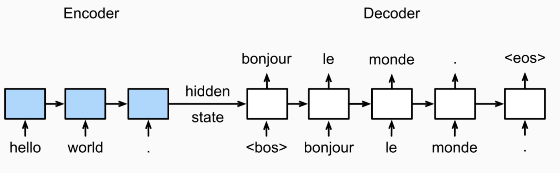
Neural machine translation (NMT) (e.g. translating from one language to another) is a way to do machine translation with a single end-to-end neural network. The neural network architecture is called sequence-to-sequence model (AKA seq2seq) and it involves two RNNs.
The job of the seq2seq model is to translate an input sequence of words (encoder) into another translated sequence of words (decoder).
It utilizes an encoder-decoder artchitecture:
- The encoder is an RNN to read the input sequence (source language).
- The decoder is another RNN to generate output word by word.
A decoder is a conditional language model; it is a language model since it is predicting the next word of the target sequence, and it is conditional because the predictions are also conditioned on the source sentence through $h^{enc}$ (encoded hidden state).
Encoder RNN:
- Word embeddings $\mathbf{E}^{(s)}$ for source language.
- RNN parameters, e.g. $\lbrace \mathbf{W},\mathbf{u},\mathbf{b}\rbrace$ for simple RNNs and $4\times$ parameters for LSTMs.
- Encoder RNN can be bidirectional.
Decoder RNN:
- Word embeddings $\mathbf{E}^{(t)}$ for target language.
- RNN parameters, e.g. $\lbrace\mathbf{W},\mathbf{U},\mathbf{b} \rbrace$, for simple RNNs and $4\times$ parameters for LSTMS.
- Outputembedding matrix $\mathbf{W}_o$ can be tied with $\mathbf{E}^{(t)}$.
- Decoder RNN has to be unidirectional (left to right).
Note that the encoder and decoder have separate word embeddings, and the encoder and decoder’s parameters are optimized together.
Sequence-tosequence is useful for more than just MT. Many NLP tasks can be framed as sequence-to-sequence problems: summarization (long text to short text), dialogue (previous utterances to next utterance), code generation (natural lange to Python code).
One problem with seq2seq is that there is a bottleneck with information, the only way the encoder has information is through the hidden state. A single encoding vector $h^{enc}$ needs to capture all the information about source sentence, and longer sequences can lead to vanishing gradients.
Attention provides a solution to the bottleneck problem. The key idea is: instead of just passing information through a single hidden layer, what if the encoder can look at all of the hidden states of the whole source sequence and decide which ones is more important?
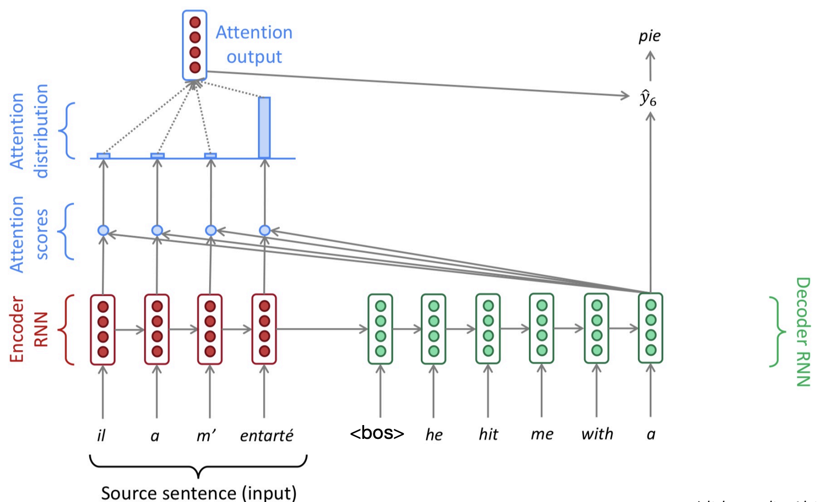
At each time step during decoding, we focus on a particular part of the source sentence. This depends on the deocder’s current hidden state $h_t^{dec}$ (i.e. an idea of what you are trying to decode), and it is usually implemented as a probability distribution over the hidden states of the encoder ($h_i^{enc}$).
In the encoder RNN, we assign attention scores at each hidden state, in order to answer - which tokens are likely to be relevant for the token I’m trying to predict?
Computing attention
Let the encoder hidden states be denoted by $h^{\text{enc}}_1, \dots, h^{\text{enc}}_n$, and let the decoder hidden state at time step $t$ be $h^{\text{dec}}_t$.
At decoding step $t$, we first compute the attention scores between the current decoder hidden state and each encoder hidden state. These scores are given by
\[e_t = \big[ g(h^{\text{enc}}_1, h^{\text{dec}}_t), \dots, g(h^{\text{enc}}_n, h^{\text{dec}}_t) \big],\]where $g(\cdot,\cdot)$ is a scoring function that measures the compatibility between encoder and decoder states.
Next, we normalize these scores using a softmax function to obtain the attention distribution:
\[\alpha_t = \text{softmax}(e_t) \in \mathbb{R}^n.\]This produces a probability distribution over the encoder time steps.
Using these attention weights, we compute a context vector as the weighted sum of the encoder hidden states:
\[a_t = \sum_{i=1}^{n} \alpha_{t,i} \, h^{\text{enc}}_i \in \mathbb{R}^h.\]We then concatenate the context vector $a_t$ with the decoder hidden state $h^{\text{dec}}_t$, apply a linear transformation followed by a $\tanh$ activation:
\[\tilde{h}_t = \tanh\!\big( W_c [a_t ; h^{\text{dec}}_t] \big),\]where $W_c \in \mathbb{R}^{2h \times h}$.
Finally, we compute the output distribution over the vocabulary by applying a linear transformation and softmax:
\[\hat{y}_t = \text{softmax}(W_o \tilde{h}_t).\]Assuming encoder hidden states $h_1^{enc},\dots,h_n^{enc}$ and a decoder hidden state $h_t^{dec}$, there are different types of attention:
- Dot-product attention, $g(h^{\text{enc}}_i, h^{\text{dec}}_t) = (h^{\text{dec}}_t)^{\top} h^{\text{enc}}_i \in \mathbb{R}$. .
- Multiplicative attention, $g(h^{\text{enc}}_i, h^{\text{dec}}_t) = (h^{\text{dec}}_t)^{\top} W \, h^{\text{enc}}_i \in \mathbb{R}$, where $W$ is a (learned) weight matrix.
- Additive attention, $g(h^{\text{enc}}_i, h^{\text{dec}}_t) = v^{\top} \tanh\big( W_1 h^{\text{enc}}_i + W_2 h^{\text{dec}}_t \big) \in \mathbb{R}$, where $W_1$, $W_2$ are (learned) weight matrices and $v$ is a (learned) weight vector.
Studies found that putting in attention into the model improves translation.
With attention we don’t have any extra parameters, it is something which is learned from the model.
Lecture 8
Self-attention and Transformers
Recall the encoder / decoder hidden states model from last time. For example. The econder could be ‘encoding’ English and the decoder generating French. But this had a bottleneck problem. Attention allows the decoder to acces the encoder hidden states for all time stamps, and hence addresses the bottleneck problem. We can form attention scores:
\[e^t = [g(h_1^{enc},h_t^{dec}),\dots,g(h_n^{enc}, h_t^{dec})]\in\mathbb{R}^n.\]The attention distribution $\alpha_t$ and weighted sum of encoder hidden states:
\[a_t = \sum_{i=1}^{n} \alpha_{t,i} \, h^{enc}_i \in \mathbb{R}^h,\quad\alpha_t = \text{softmax}(e_t) \in \mathbb{R}^n.\]We combine $a_t$ and $h_t^{dec}$ to predict the next word.
We can think of attention as performing fuzzy lookup in key-value store. While a lookup table takes a query, matches one of the keys and returns its value, attention takes the query, matches to all keys softly to a weight between $0$ and $1$. The keys’ value are mupltiplied by the eights and summed. Thus, in a way, attention is weighted average of these keys.
We don’t completely need the RNN using attention (famous paper: “Attention is all you need”). Transformers don’t have any recurrence structures!
\[\mathbf{h}_t = f(\mathbf{h}_{t-1}, \mathbf{x}_t) \in \mathbb{R}^h\]Transformer encoder is a stack of encoder layers. Transformer decoder is a stack of decoder layers. Examples of transformer encoder models are BERT, ELECTRA; and examples of transformer decoder models are GPT-3, ChatGPT, Palm. Examples of transformer encoder-decoder
The main innovation is multi-head and self-attention (to be explained).
The issues with recurrent NNs, is that longer sequences can lead to vanishing gradients, i.e. it is hard to capture long-distance information. Moreover, RNNs lack parallelizability, since forward and backward passes have $O(\text{sequence length})$ unparallelizable operations. Transformers are much easier to parallelize (hence these models can be trained much faster on large datasets on GPUs).
History:
RNNs / LSTMs → seq2seq → seq2seq + attention → attention only = Transformers!
Attention in a general form
Assume that we have set of keys and values $(\mathbf{k}_1,\mathbf{v}_1),\dots,(\mathbf{k}_n,\mathbf{v}_n)$, $\mathbf{k}_i\in\mathbb{R}^{d_k}$, $\mathbf{v}_i\in\mathbb{R}^{d_v}$. Keys are used to compute the attention scores and values are used to compute the output vector.
Attention always involves the following steps:
-
Compute the attention score $\mathbf{e} = g(\mathbf{q},\mathbf{k}_i)\in\mathbb{R}^n$ (observe that attention scores are invariant to the ordeering of the words).
-
Taking softmax to get attention distribution $\alpha$:
Using the attention distribution to compute the weighted sum of values:
\[a = \sum_{i=1}^{n} \alpha_i v_i \in \mathbb{R}^{d_v}.\]Self-attention
In NMT, the query is the decoder hidden state, and the keys are equal to the values which are equal to the encoder hidden states.
Self-attention is attention from the sequence to itself. In self-attention, we say: ‘let’s use each word in a sequence as the query, and all the other words in the sequence as keys and values’.
A self-attention layer maps a sequence of input vectors $\mathbf{x}_1,\dots,\mathbf{x}_n\in\mathbb{R}^{d_1}$ to a sequence of $n$ vectors: $\mathbf{h_1},\dots,\mathbf{h}_n\in\mathbb{R}^{d_2}$.
We have the same abstraction as RNNs - this is used as a drop-in replacement for an RNN layer,
\[\mathbf{h}_t = g(\mathbf{W}\mathbf{h}_{t-1} + \mathbf{U}\mathbf{x}_t+\mathbf{b})\in\mathbb{R}^h.\]Self-attention:
\[\mathbf{q}_i = \mathbf{W}^{(q)} \mathbf{x}_i, \quad \mathbf{k}_i = \mathbf{W}^{(k)} \mathbf{x}_i, \quad \mathbf{v}_i = \mathbf{W}^{(v)} \mathbf{x}_i\] \[\mathbf{h}_i = \mathbf{W}^{(o)} \sum_{j=1}^{n} \left( \frac{ \exp\left( \mathbf{q}_i \cdot \mathbf{k}_j / \sqrt{d} \right) }{ \sum_{j'=1}^{n} \exp\left( \mathbf{q}_i \cdot \mathbf{k}_{j'} / \sqrt{d} \right) } \mathbf{v}_j \right)\] \[\text{where } \mathbf{W}^{(q)}, \mathbf{W}^{(k)}, \mathbf{W}^{(v)}, \mathbf{W}^{(o)} \in \mathbb{R}^{d \times d}.\]We will break this down.
First step is to transform each input vector in three vectors: query, key and value vectors.
\[\mathbf{q}_i = \mathbf{x}_i \mathbf{W}^Q \in \mathbb{R}^{d_q}, \quad \mathbf{k}_i = \mathbf{x}_i \mathbf{W}^K \in \mathbb{R}^{d_k}, \quad \mathbf{v}_i = \mathbf{x}_i \mathbf{W}^V \in \mathbb{R}^{d_v}\] \[\mathbf{W}^Q \in \mathbb{R}^{d_1 \times d_q}, \quad \mathbf{W}^K \in \mathbb{R}^{d_1 \times d_k}, \quad \mathbf{W}^V \in \mathbb{R}^{d_1 \times d_v}\]The second step is to compute pairwise simlarities between keys and queries; then normalize with softmax. For each $\mathbf{q}_i$, we compute attenion scores and attention distribution:
\[\alpha_{i,j} = \operatorname{softmax}\left( \frac{\mathbf{q}_i\cdot\mathbf{k}_j}{\sqrt{d_k}}\right).\]The above is the scaled dot product. The intuition for using this is assuming $q_i$, $k_j$ are normally distributed, the dot product might be too large for larger $d_k$; scaling the dot product by $\frac{1}{\sqrt{d_k}}$ is easier for optimization.
The third step is to compute the output for each input as weighted sum of values,
\[\mathbf{h}_i = \sum_{j=1}^n\alpha_{i,j}\mathbf{v}_j\in\mathbb{R}^{d_v}.\]We can write self-attention succinctly in matrix notation.
\[X \in \mathbb{R}^{n \times d_1} \quad (n = \text{input length})\] \[Q = XW^Q, \quad K = XW^K, \quad V = XW^V\] \[W^Q \in \mathbb{R}^{d_1 \times d_q}, \quad W^K \in \mathbb{R}^{d_1 \times d_k}, \quad W^V \in \mathbb{R}^{d_1 \times d_v}\] \[\mathrm{Attention}(Q, K, V) = \mathrm{softmax} \left( \frac{QK^{T}}{\sqrt{d_k}} \right) V\]Multi-head attention
It is better to use mutliple attention functions instead of just one. Each attention function (‘head’) can focus on different key positions / content. For different attention heads, we are using different matrices to $Q$, $K$, $V$. (Typically, $16$, $32$, $64$ heads used - larger models will have more heads.)
Finally, we just concatenate all the heads and apply an output projection matrix, i.e. run a bunch of them and concatenate the output.
\[\begin{aligned} \text{MultiHead}(Q, K, V) &= \mathrm{Concat}(\mathrm{head}_1, \ldots, \mathrm{head}_h) W^O \\ \mathrm{head}_i &= \mathrm{Attention}(X W_i^Q, X W_i^K, X W_i^V) \end{aligned}\]In practice, we use a reduced dimension for each head.
\[W_i^Q \in \mathbb{R}^{d_1 \times d_q}, \; W_i^K \in \mathbb{R}^{d_1 \times d_k}, \; W_i^V \in \mathbb{R}^{d_1 \times d_v}, \quad d_q = d_k = d_v = d/m.\]$d$ is the hidden size, $m$ is the number of heads. $W_o\in\mathbb{R}^{d\times d_2}$ has those dimensions, and if we stack multiple layers, we usually get $d_1=d_2=d$.
Earlier we saw attention scores are positional invariant (it doesn’t care what order words come in). The fix is to add a positional encoding (not unlike word embedding).
Unlike RNNs, self-attention doesn’t build in order information, we need to encode the order of the sentence in our keys, queries and values.
The solution is to add positional encodings to the input embeddings, $\mathbf{p}_i\in\mathbb{R}^d$ for $i=1,2,\dots,n$, $\mathbf{x}\leftarrow\mathbf{x}_i+\mathbf{p}_i$.
We can use learned absolute position encodings: let all $\mathbf{p}_i$ be learnable parameters. Similar to word embeddings, $P\in\mathbb{R}^{d\times L}$ for $L=$ max sequence length.
The pros of this are that each position gets to be learned to fit the data, while the cons are that it can’t extrapolate to indices outside of max sequence length $L$.
So far if you only have attention, it looks like attention is just taking average of words. There are no element-wise nonlinearities in self-attention; stacking more self-attention layers just re-averages value vectors.
The simple fix to this is to add a feed-forward network to post-process each output vector.
\[\begin{aligned} \mathrm{FFN}(x_i) &= \mathrm{ReLU}(x_i W_1 + b_1) W_2 + b_2 \\ W_1 \in \mathbb{R}^{d \times d_{ff}}&, b_1 \in \mathbb{R}^{d_{ff}}, W_2 \in \mathbb{R}^{d_{ff} \times d}, b_2 \in \mathbb{R}^{d} \end{aligned}\]This is actually where the majority of the compute and parameters go.
Transformer encoder: putting things together
The way you read this architecture is from the bottom - to the top.
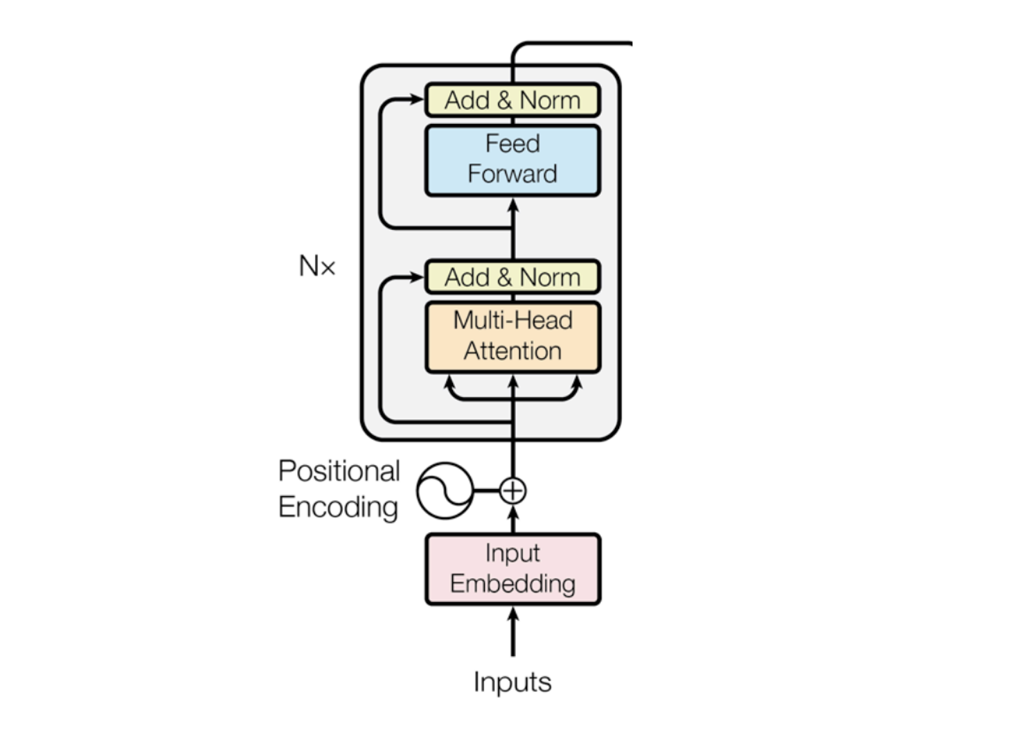
Input (bunch of words) turn them into vectors with embedding and add positional encoding. Then you stack a bunch of layers - transformer encoder is a stack of $N$ layers (each of the layers will have $2$ sub layers: the multi-head layer and the feedforward layer). The way these $2$ layers are connected is through add & norm.
These models are sequence2sequence; turn one sequence of vectors into another sequence of vectors.
Add & Norm is also known as ‘residual connection and layer normalization’,
\[\text{LayerNorm}(x+\text{Sublayer}(x)).\]Instead of $X^{(i)}=\text{Layer}(X^{(i-1)})$ ($i$ represents the layer), we let $X^{(i)}=X^{(i-1)}+\text{Layer}(X^{(i-1)})$, so we only need to learn the ‘residual’ from the previous layer.
The layer normalization is applied, which helps train the model faster. The ideas is to normalize the hidden vector values to unit mean and standard deviation within each layer.
\[y = \frac{x - \mathbb{E}[x]}{\sqrt{\mathrm{Var}[x] + \epsilon}} \, \gamma + \beta, \quad \gamma, \beta \in \mathbb{R}^d \text{ are learnable parameters.}\]Lecture 9
Self-attention II
Self-attention ($Q$, $K$, $V$)
A self-attention layer maps a sequence of input vectors to a sequence of $n$ output vectors:
- Inputs: $\mathbf{x}_1,\dots,\mathbf{x}_n \in \mathbb{R}^{d_1}$ .
- Outputs: $\mathbf{h}_1,\dots,\mathbf{h}_n \in \mathbb{R}^{d_2}$.
First step is to transform each input into three query, key, value vectors.
\[\mathbf{q}_i = \mathbf{x}_i \mathbf{W}^Q \in \mathbb{R}^{d_q},\quad \mathbf{k}_i = \mathbf{x}_i \mathbf{W}^K \in \mathbb{R}^{d_k},\quad \mathbf{v}_i = \mathbf{x}_i \mathbf{W}^V \in \mathbb{R}^{d_v}\] \[\mathbf{W}^Q \in \mathbb{R}^{d_1 \times d_q},\quad \mathbf{W}^K \in \mathbb{R}^{d_1 \times d_k},\quad \mathbf{W}^V \in \mathbb{R}^{d_1 \times d_v}\]Next, we compute pairwise similarities between keys and queries, and normalize with softmax.
For each query $\mathbf{q}_i$, compute attention scores and attention distribution against all keys:
\[e_{i,j} = \frac{\mathbf{q}_i \cdot \mathbf{k}_j}{\sqrt{d_k}},\quad \forall j=1,\dots,n\] \[\alpha_i = \mathrm{softmax}(\mathbf{e}_i),\quad \alpha_{i,j} = \frac{\exp(e_{i,j})}{\sum_{k=1}^{n}\exp(e_{i,k})}.\]The final step is to take the weighted sum of these values, $h_i = \sum_{j=1}^{n}\alpha_{i,j} v_j$.
In a matrix view, we have (same idea), $Q = XW^Q$, $K = XW^K$, $V = XW^V$.
\[\mathrm{Attention}(Q,K,V)=\mathrm{softmax}\!\left(\frac{QK^\top}{\sqrt{d_k}}\right)V\]Putting things together, for a transformer encoder (stack of $N$ layers), from the bottom to top we have:
- Input embedding
- Positional encoding
- A stack of transformer encoder layers
Each encoder layer has two sub-layers: multi-head attention and feed-forward, with add & norm between sub-layers.
Overall:
\[x_1,\dots,x_n \in \mathbb{R}^{d_1} \to h_1,\dots,h_n \in \mathbb{R}^{d_2}\]For a transformer decoder (stack of $N$ layers), we have, from bottom to top:
- Output embedding
- Positional encoding
- A stack of transformer decoder layers
- Linear + softmax (to produce output probabilities)
Each decoder layer has three sub-layers:
- Masked multi-head (self-) attention (within target sequence)
- Multi-head cross-attention (between source and target sequences)
- Feed-forward
- (With add & norm between sub-layers)
Masked multi-head attention
In the decoder, when predicting the next token, we must not look at future tokens. That is, at position $i$, we are only allowed to attend to positions $j \le i$. This is called masked (or causal) self-attention in the decoder.
Formally, the attention mechanism is the same as usual self-attention:
\[\mathbf{q}_i = \mathbf{x}_i \mathbf{W}^Q,\quad \mathbf{k}_j = \mathbf{x}_j \mathbf{W}^K,\quad \mathbf{v}_j = \mathbf{x}_j \mathbf{W}^V\] \[e_{i,j}=\frac{\mathbf{q}_i\cdot \mathbf{k}_j}{\sqrt{d_k}}\]but the key difference is: we mask out all scores where $j>i$.
Let $M\in\mathbb{R}^{n\times n}$ be a causal mask (set future scores to $-\infty$),
\[M_{i,j}= \begin{cases} 0 & \text{if } j\le i\\ -\infty & \text{if } j>i \end{cases}.\]Then we apply the mask before softmax,
\[\alpha_i = \mathrm{softmax}(e_i + M_i).\]Equivalently, for $j>i$, $e_{i,j}=-\infty$, so after softmax,
\[\alpha_{i,j}=0 \quad \text{for all } j>i.\]Finally, the output is the same weighted sum,
\[\mathbf{h}_i=\sum_{j=1}^{n}\alpha_{i,j}\mathbf{v}_j, \quad \text{but only } j\le i \text{ contribute.}\]For position $i$, attention becomes a distribution over only the prefix $(1,\dots,i)$.
This enforces autoregressive generation: when predicting token $i$, the model can only use tokens $< i$.
During training, masking is what allows the decoder to compute all positions in parallel without leaking future information.
Masked attention is applied independently per head. Each head has its own projections $W_h^Q, W_h^K, W_h^V$, but the same causal mask is used in every head.
The key idea is that: multi-head gives multiple “views” of the prefix, and masking ensures no head can access the future.
Multi-head cross-attention
Cross-attention is the mechanism that lets the decoder look at the encoder outputs (i.e. the source sequence) while generating the target sequence. It is the “bridge” between the encoder and decoder stacks. This is why this is AKA encoder-decoder attention.
We have encoder top-layer outputs (source representations): $\tilde{\mathbf{x}}_1,\dots,\tilde{\mathbf{x}}_m$.
And, decoder current-layer inputs (target-side representations): $\mathbf{x}_1,\dots,\mathbf{x}_n$.
The crucial distinction from self-attention is that:
- Queries come from the decoder states $\mathbf{x}_i$.
- Keys and values come from the encoder states $\tilde{\mathbf{x}}_j$.
For each decoder position $i$, define, $\mathbf{q}_i = \mathbf{x}_i \mathbf{W}^Q$, and for each encoder position $j$, define,
\[\mathbf{k}_j = \tilde{\mathbf{x}}_j \mathbf{W}^K,\quad \mathbf{v}_j = \tilde{\mathbf{x}}_j \mathbf{W}^V.\]We then compute scaled dot-product scores,
\[e_{i,j} = \frac{\mathbf{q}_i \cdot \mathbf{k}_j}{\sqrt{d_k}},\quad j=1,\dots,m.\]Normalize over the encoder positions,
\[\alpha_i = \mathrm{softmax}(\mathbf{e}_i),\quad \alpha_{i,j} = \frac{\exp(e_{i,j})}{\sum_{k=1}^{m}\exp(e_{i,k})}.\]Then, we form the context vector / output,
\[\mathbf{h}_i = \sum_{j=1}^{m}\alpha_{i,j}\mathbf{v}_j.\]The interpretation is that at each decoder position $i$, the model computes a distribution over source tokens and then takes a weighted sum of their value vectors.
With multi-head self-attention, we run several cross-attention heads in parallel. Each head uses its own learned projections:
For head $h$,
\[Q_h = X W_h^Q,\quad K_h = \tilde{X} W_h^K,\quad V_h = \tilde{X} W_h^V,\]and
\[\text{head}_h = \mathrm{Attention}(Q_h, K_h, V_h) = \mathrm{softmax}\!\left(\frac{Q_h K_h^\top}{\sqrt{d_k}}\right)V_h.\]Then, concatenate and project,
\[\mathrm{CrossMultiHead}(Q,K,V)=\mathrm{Concat}(\text{head}_1,\dots,\text{head}_H)\,W^O.\]Lecture 10
Contexualized Representations and Pre-training
Contexualized word embeddings
We previously saw ‘word2vec’, which gave us one vector for each word type (i.e. static embeddings). This is a limitation, since one word can have multiple meanings, which is dependent on context.
The idea of contexualized word embeddings is to build a vector for each word conditioned on its context. Instead of treating a vector that is static for every word, let’s make it more dynamic. We look at the context where each word appears.
A contexualized embedding is simply: a word representation that changes depending on the sentence it appears in.
Now we take all the words as input, and give a set of vectors produced for all the words in that context.
\[f: (w_1,\dots,w_n)\to \mathbf{x}_1,\dots,\mathbf{x}_n\in\mathbb{R}^d\]ELMo (Embeddings from Language Model) is one such contexualized word embedding models.
Whenever we talk about context, we are dealing with sequences; we take a sequence of inputs and output a sequence of vectors. The key of idea is ELMo is to train two stacked LSTM-based (specific type of RNN) language models on a large corpus.
\[\mathrm{ELMo}_k^{\text{task}} = E\!\left(R_k; \Theta^{\text{task}}\right) = \gamma^{\text{task}} \sum_{j=0}^{L} s_j^{\text{task}} \mathbf{h}_{k,j}^{\text{LM}}\]This saying that the contexualized word embeddding is the weighted average of input embeddings $h_0$ and all hidden representations $h_j$. The weights $\gamma^{\text{task}}$, $s_j^{\text{task}}$ here are task-dependent and learned.
We run the forward LSTM model and the backward LSTM model, and first concatenate the hidden layers (so we get $2$ of each layers).
Then, we multiply each layer vector by a weight $s_i$ based on the task (different tasks will use different embeddings from each of the layers, e.g. for something like semantic analysis for example, maybe the lower layers might matter more than the higher layers).
Finally, we sum the (now) weighted vectors.
For pre-training ELMo, they used $10$ epochs on $1$B Word Benchmark, and so every data point for training is going to be a single sentence. The training time is $2$ weeks on $3$ NVIDIA GTX 1080 GPUs.
We use both forward and backward language models, because it is important to model both left and right context; bidirectionality is very important in language understanding tasks.
Moreover, we use the weighted average of different layers instead of just the top layer, since different layers are expected to encode different information.
Note that ELMo takes as input a vector of each of the different words. Each word’s input vector is built from its characters, not from a pre-trained word embedding: the characters are embedded, passed through a character-level CNN with max pooling to produce a fixed-length vector capturing morphological patterns.
This vector is then fed into a bidirectional LSTM language model, which generates the final context-dependent word representation.
Pre-training and fine-tuning
Suppose we have a large dataset for task $X$, train this model on dataset $X$, then we can take the whole model and ‘fine-tune’ or further train it on a dataset for task $Y$. The key idea is that if $X$ is somewhat related to $Y$, a model that can do $X$ will have some good neural representations for $Y$ as well.
Can we find some task $X$ (e.g. computer vision ImageNet) that can be useful for a wide range of downstream tasks $Y$? We end up taking the same original neural network, although we may add a few parameters on top.
ELMo is a feature-based approach which only produces word embeddings that can be used as input representations of existing neural models.
GPT/BERT (and most of following models) are fine-tuning approaches. Almost all model weights will be reused, and only a small number of task-specific will be added for downstream tasks. You’re not training the ELMO word embeddings - you are just ‘fine-tuning’ them.
In ELMo, contextualized representations are produced by stacking bidirectional LSTMs, where each word’s representation is updated sequentially using left and right context. In transformer models like BERT, contextualization instead happens through stacked self-attention layers, where each token directly attends to all other tokens in the sequence at every layer.
The neural architecture influences the type of pre-training and natural use cases:
- Encoders: gets bidirectional context.
- Encoder-decoders: gets good parts of encoders and decoders?
- Decoders: language models.
For example, if you have a transformer-encoder, how can we pre-train it to do well on a particular task?
BERT (Bidirectional Encoder Representations from Transformers, released in 10/2018) is a fine-tuning approach based on a deep bidirectional transformer encoder instead of a transformer decoder.
The key is to learn representations based on bidirectional contexts.
There are two new pre-training objectives:
- Masked language modelling (MLM).
- Next sentence prediction (NSP), although later work showed NSP hurts performance.
We can’t do language modelling with bidirectional models since they ‘cheat’ by looking at future words when predicting a token, whereas true language modeling requires predicting each word using only past context so the model can generate text step by step without knowing the future.
The solution to this is to mask out $k\%$ of the input words, and then predict the masked words. In practice $k=15\%$.
e.g. the man went to [MASK] to buy a [MASK] of milk. Here, we have masked words: ‘store’ and ‘gallon’. [MASK] tokens are never seen during fine-tuning.
BERT just used a simple transformer encoder - why not use pre-trained encoders for everything? If your task involves generating sentences, BERT and other pre-trained encoders don’t naturally lead to nice autoregressive ($1$-word-at-a-time) generation methods.
The alternative to using the encoder is to use the decoder (autoregressively generates one token at a time).
GPT (Generative Pre-Training, released in 06/2018) uses a transformer decoder (unidirectional; left-to-right) instead of LSTMs. We use language modeling as a pre-training objective. This is trained on longer segments of text, not just single sentences.
One you have a decoder only model, we can fine-tune the entire set of model parameters on various downstream tasks, e.g. classification, entailment, similarity etc.