ECE 530
Signal Detection & Estimation
Written live in classes with Prof. Vince Poor (and closely following his book, An Introduction to Signal Detection and Estimation).
Last updated: 02/26.
Contents
- Introduction
- Bayesian Hypothesis Testing
- Minimax Hypothesis Testing
- Neyman-Pearson Hypothesis Testing
- Composite Hypothesis Testing
- Signal Detection
Lecture 1
Introduction
We have a random observation $Y$ and we wish to process it to extract some underlying information.
There are two exaples: $Y = (Y_1, Y_2,\dots,Y_n)^\top$, or $Y$ is an element of a discrete set.
\[\implies \Gamma=\text{ observation set }=\begin{cases}\mathbb{R}^n \text{ or}\\ \{\gamma_1, \gamma_2,\dots\}\end{cases}\]We want to assign probabilities to subsets of $\Gamma$.
If $\Gamma$ is discrete, probabilities can be assigned via a probability mass function (pmf), $p:\Gamma\to [0,1]$.
\[p(A) = \sum_{\gamma_i\in A} p(\gamma_i),\quad p(\gamma_i) = P(Y=\gamma_i),\quad i=1,2,\dots\]If $\Gamma=\mathbb{R}^n$, we need to specify an event class $\mathcal{G}$, i.e. a set of subsets of $\Gamma$ that we can assign probabilities to with these properties:
- if $A\in\mathcal{G}$, the so is $A^C$.
- if $A_1,A_2,\dots\in\mathcal{G}$, then $A_1\cup A_2\cup\dots\in\mathcal{G}$.
A set $\mathcal{G}$ with these properties is called a $\sigma$-field ($\sigma$-algebra).
For discrete $\gamma$, $\mathcal{G}$ can be the set of all subsets of $\Gamma$, $2^\Gamma$.
\(\{y\in\mathbb{R}^n|y_1\in [a_,b_1], y_2\in[a_2,b_2],\dots,y_n\in[a_n,b_n]\}\quad \forall a_i,b_i\) This is the smallest $\sigma$-field that contains all such sets called the Borel field in $\mathbb{R}^n$, and we write it $\mathbb{B}^n$.
For $\Gamma=\mathbb{R}^n$, we’re going to consider only continuous random vectors, so that there will be a probability density function (pdf) $p:\mathbb{R}^n\to [0,\infty)$, so that $P(A) = \int_A p(y)dy$, $A\in\mathbb{B}^n$.
For discrete $\Gamma$, any $p:\Gamma\to [0,1]$ is a legitimate pmf if $\sum_{i=1}^\infty p(\gamma_i) = 1$.
For continuous $\Gamma$, any integrable $p:\Gamma\to [0,\infty)$ is a legit pdf if $\int_{\mathbb{R}^n} p(y)dy = 1$.
To avoid switching between discrete and continuous throughout the course, we use the notation $P(A) = \int_A p(y)\mu(dy)$ (Lebesgue integral analogue) for both.
We’re also interested in expected values of functions of $Y$, say $g(Y)$, where $g:\Gamma\to\mathbb{R}$.
- $\Gamma$ is discrete: $E{g(Y)} = \sum_{i=1}^\infty g(\gamma_i) p(\gamma_i)$.
- $\Gamma=\mathbb{R}^n$: $E{g(Y)} = \int_{\mathbb{R}^n} g(y)p(y)dy$.
Again, to cover both cases, we’ll write $E{g(Y)} = \int_\Gamma g(y)p(y)\mu(dy) = \int_\Gamma gp\mathrm{d}\mu$.
To clarify, $\Gamma$ is observation set, $\mathcal{G}$ is event class, $(\Gamma,\mathcal{G})$ is observation space.
Notation: uppercase letters denote random quantities, say $Y$; lowercase letters denote specific values of random quantities, say $y$.
Lecture 2
Last time we set up a structure of an observation set $\Gamma$, event class $\mathcal{G}$, random observation $Y$, and $y$ - a specific observation of $Y$.
We also recall the notation for a function $g:\Gamma\to\mathbb{R}$, with its expectation $E{g(Y)} = \int_\Gamma g(y)p(y)\mu(dy)=\int_\Gamma gp\mathrm{d}\mu$, in terms of the probability density $p$.
We will look at hypothesis testing - the situation where observing $y$ (assuming finite number of states of nature), and make a decision on which one of those is true.
Hypothesis testing
There are $M$ ‘states of nature’ or ‘hypotheses’
We’ll focus on the binary case, $M=2$: binary hypothesis testing. The two hypotheses correspond to two probability distributions on $P_0$ and $P_1$, i.e. if $H_j$ (the $j$-th hypothesis) is true then $Y\sim P_j$.
We can write this as $H_0$: $Y\sim P_0$ vs. $H_1$: $Y\sim P_1$, where $Y\sim P$ means $Y$ has distribution $P$.
We define a decision rule $\delta$ is a partition of $\Gamma$ into $\Gamma_1$ and $\Gamma_0=\Gamma_1^C$, s.t. if $y\in\Gamma_1$, we announce that $H_1$ is true, and if $y\in\Gamma_0$, we announce $H_0$ is true.
In statistics jargon, $\Gamma_1$ is often called the ‘rejection region’ (or ‘critical region’), and $\Gamma_0$ the ‘acceptance region’.
We can also think of $\delta$ as a function on $\Gamma$, $\delta:\Gamma\to {0,1}$ s.t. \(\delta(y) = \begin{cases}1,\quad \text{if }y\in\Gamma_1, \\ 0,\quad \text{if }y\in\Gamma_0 \end{cases} = \text{`indicator function of }\Gamma_1\text{'}.\)
We need to assing costs, in order to optimize for making mistakes etc. Assign costs $C_{ij}$, which is the cost of choosing $H_i$ when $H_j$ is true, for $i,j\in{0,1}$.
Given costs, we can define conditional risks associated with a decision rule $\delta$: \(R_j(\delta) = C_{1j}P_j(\Gamma_1) + C_{0j}P_j(\Gamma_0),\quad j=0,1.\)
All types of hypothesis testing we’re going to talk about (e.g. minimax, Neyman-Pearson) are just different ways of trading off these (two) conditional risks.
One way of trading these off is to average them over prior probabilities $\pi_0$ and $\pi_1=1-\pi_0$ of $H_0$ and $H_1$ occurring. $\pi_1$ is the probability that $H_j$ is true unconditioned on the value of $Y$.
We’d like to choose $\delta$ to minimize the average risk $r(\delta) = \pi_0R_0(\delta)+\pi_1R_1(\delta)$ (AKA the Bayes risk).
An optimal decision rule is one that minimizes $r(\delta)$.
\[\begin{align*} r(\delta) &= \sum_{j=0}^1 \pi_j \left[C_{0j}\overbrace{(1-P_j(\Gamma_1))}^{P_j(\Gamma_0)} + C_{1j}P_j(\Gamma_1) \right] \\\\ &= \sum_{j=0}^1 \pi_1C_{0j} + \sum_{j=0}^1\pi_j(C_{ij} - C_{0j})P_j(\Gamma_1) \end{align*}\]Assume $P_0$ and $P_1$ have densities $p_0$ and $p_1$. Then,
\[r(\delta) = \sum_{j=0}^1 \pi_1 C_{0j} + \int_{\Gamma_1}\sum_{j=0}^1\pi_j(C_{1j} - C_{0j})p_j(y)\mu(dy).\]So, an optimal choice of $\Gamma_1$ is,
\[\begin{align*} \Gamma_1 &= \{y\in\Gamma \mid \sum_{j=0}^1 \pi_j(C_{ij}-C_{0j})p_j(y)\le 0 \} \\ &= \{ y\in\Gamma \mid \pi_1(C_{11} - C_{01})p_1(y) \le \pi_0(C_{00} - C_{10})p_0(y) \} \end{align*}\]For intuition on the line above: the inequality is basically saying if the average (or posterior) cost of $H_1$ is less than the average cost of $H_0$, then we pick $H_1$.
If we assume $C_{11} < C_{01}$ then,
\[\Gamma_1 = \{y\in\Gamma \mid p_1(y)\ge \tau p_0(y)\},\quad \tau = \frac{\pi_0(C_{10}-C_{00})}{\pi_1(C_{01} - C_{11})}.\]$\tau$, here, is controlling for what it costs to make mistakes.
(Note that in this situation we have a model $P_1$, $P_0$ - but when we don’t have a model we need machine learning (see later in the course).)
We can further write $\Gamma_1 = {y\in\Gamma \mid L(y)\ge \tau }$ (‘likelihood ratio test’), where $L(y)=\frac{p_1(y)}{p_0(y)}$ is the likelihood ratio.
So, the Bayes rule is just $\delta_B(y)=\begin{cases}1\text{, if }L(y)\ge\tau \ 0 \text{, if }L(y) <\tau \end{cases}$.
A common cost criterion is uniform costs: $C_{ij}$ equals $1$ if $i\neq j$, and $0$ if $i=j$. It costs zero to get the answer right and it cost 1 to make the answer wrong.
In this case, the Bayes risk is $r(\delta) = \pi_0P_0(\Gamma_1) + \pi_1P_1(\Gamma_0)$, equal to the average probability of error. This is because the second term is the probability we make an error under $H_1$, and the first term is probability make an error under $H_0$.
Here, $\tau=\frac{\pi_0}{\pi_1}\notin\delta_B$ is the minimum probability of error decision rule.
Bayes’ formula: ‘posterior probability’ of $H_j$ is
\[\pi_j(y) = P(H_j\text{ is true} \mid Y=y) = \frac{p_j(y)\pi_j}{p(y)},\quad j=0,1,\]where $p(y)=\pi_0p_0(y)+\pi_1p_1(y)$ is average density ,since $\pi_0$ is probability of $p_0(y)$ occuring etc.
So, a conclusion is that the Bayes test depends only on the posterior probabilities of the hypotheses given the observation.
For uniform costs, the Bayes rule can be written $\delta_B(y) = \begin{cases}1 \text{ if }\pi_1(y)\ge\pi_0(y)\ 0 \text{ if }\pi_1(y) < \pi_0(y)\end{cases}$ (the minimum error probability decision rule, choosing the hypothesis that has maximum posterior probability of having occurred given $Y=y$).
Examples
Binary channel (discrete) - suppose a binary digit ($0$ or $1$) is to be transmitted over a channel, but imperfect so transmitted ‘$0$’ is received as $1$ with probability $\lambda_0$. And, transmitted ‘$1$’ received as a $0$ with probability $\lambda_1$ (and $1$ with probability $1-\lambda_1$ of course).
The hypothesis $H_j$ is that a ‘$j$’ was transmitted, observation set $\Gamma={0,1}$, and the observation $Y$ has densities/pmfs as follows. We define ‘crossover probabilties’,
\[p_{j}(y) = \begin{cases}\lambda_j \quad\text{ if }y\neq j\\ 1-\lambda_j\quad\text{ if } y=j \end{cases}.\]The likelihood ratio is
\[L(y) = \frac{p_1(y)}{p_0(y)} = \begin{cases}\frac{\lambda_1}{1-\lambda_0} \quad\text{ if }y=0 \\ \frac{1-\lambda_1}{\lambda_0} \quad\text{ if }y=1 \end{cases}.\]The priors and costs determine a threshold $\tau$, e.g. if uniform costs and equal priors $\tau=1$.
If $\lambda_1\ge\tau(1-\lambda_0)$, then if we observe a $0$, we say a ‘$1$’ was transmitted. If $\lambda_1<\tau(1-\lambda_0)$ and we observe $0$, we say a ‘$0$’ was transimtted.
Similarly, if $(1-\lambda_1)\ge\tau\lambda_0$ and we observe a $1$, we say ‘$1$’ was transmitted, and similar for the ‘$0$’. This is all the Bayes rule.
For the $\tau=1$ case (uniform costs and equal priors), the optimal Bayes rule may be written as
\[\delta_B(y) = \begin{cases} y,\quad 1-\lambda_1\ge\lambda_0 \\ 1-y,\quad 1-\lambda_1<\lambda_0 \end{cases}.\]For the binary symmetric channel: $\lambda_1=\lambda_0=\lambda$, this further reduces to $\delta_B(y) = \begin{cases} y,\quad \lambda\le 1/2 \\ 1-y,\quad \lambda>1/2 \end{cases}$.
The interpretation of this is: if $\lambda>1/2$ (i.e. the channel is more likely than not to invert bits), we make our decision by inverting the received bit, otherwise if less than $1/2$ we accept the received bit as being correct. In this case, it turns out that the Bayes risk is $r(\delta_B)=\min \lbrace \lambda, 1-\lambda \rbrace$.
Lecture 3
Last time we had a random observation $Y\in\Gamma$ and we had to decide which distribution it came from; $H_0: Y\sim P_0$, $H_1: Y\sim P_1$.
There were also costs $C_{ij}$, the cost of choosing $H_i$ when $H_j$ is true, and a decision rule $\delta$ which is a partition of $\Gamma$ into $\Gamma_1$ and $\Gamma_0=\Gamma_1^C$. If we observe $Y=y\in\Gamma_1$, we say $H_1$ is true and otherwise we say $H_0$ is true.
The value of $\delta$ is the index of the chosen hypothesis, i.e. $\delta(y) = 1$ if $y\in\Gamma_1$ and $0$ if $y\in\Gamma_0$. We also have ‘conditional risks’, $R_j(\delta) = C_{1j}P_j(\Gamma_1) + C_{0j}P_j(\Gamma_0)$.
We spoke about Bayesian hypothesis testing, which finds a trade-ff between $R_0(\delta)$ and $R_1(\delta)$, by assigning priors $\pi_0$ and $\pi_1=1-\pi_0$ to $H_0$ and $H_1$ and minimize $r(\delta) = \pi_0R_0(\delta)+\pi_1R_1(\delta)$ , the Bayes (or average) risk.
Assuming $C_{11}<C_{01}$, $\delta_B(y)$ is 1 if $L(y)\ge\tau$ and $0$ otherwise, where \tau is threshold and $L(y)$ is the likelihood ratio, determined by
\[L(y) = \frac{p_1(y)}{p_0(y)},\quad \tau=\frac{\pi_0}{\pi_1}\left( \frac{C_{10}-C_{00}}{C_{01}-C_{11}}\right)\]Example 2
Location testing with Gaussian error (continuous) - $\Gamma=\mathbb{R}$ $H_0:y\sim N(\mu_0,\sigma^2)$, $H_1:Y\sim N(\mu_1,\sigma^2)$, which can be written $H_0:Y=\varepsilon + \mu_0$, $H_1: Y=\varepsilon+\mu_1$.
Assume $\mu_1>\mu_0$ (doesn’t really matter much). Then the likelihood ratio is
\[L(y) = \frac{\frac{1}{\sqrt{2\pi}\sigma}e^{-(y-\mu_1)^2/2\sigma^2}}{\frac{1}{\sqrt{2\pi}\sigma}e^{-(y-\mu_0)^2/2\sigma^2}} = \exp\left\lbrace \frac{\mu_1-\mu_0}{\sigma^2}\left(y-\frac{\mu_0+\mu_1}{2}\right) \right\rbrace\]Comparing this to $\tau$ is equivalent to comparing $y$ to another threshold, since the above is a one-to-one increasing function of $y$.
We have $\delta_B(y)$ is $1$ if $y\ge\tau’$ and $0$ otherwise, where $\tau’ = \frac{\sigma^2}{\mu_1-\mu_0}\log\tau + \frac{\mu_0+\mu_1}{2}$.
For uniform costs and equal priors, $\tau=1$ and $\tau’=\frac{\mu_0+\mu_1}{2}$. So if we’re above the average of the two means we say $H_1$ is true and vice-versa.
For uniform costs, $\tau=\frac{\pi_0}{\pi_1}\left(\frac{C_{10} - C_{00}}{C_{01}-C_{11}}\right) = \frac{\pi_0}{1-\pi_0}$.
Minimax Hypothesis Testing
Another way of trading off the two conditional risks (Bayesian case where we’ve been looking at the average, if we know the priors). But what if we don’t know the priors?
$R_0(\delta_1)\notin R_1(\delta)$ - how do we design $\delta$ is we don’t have priors?
One idea is to look at the worst-case risk (or maximum risk), and minimize that over $\delta$,
\[\min_\delta \max \lbrace R_0(\delta), R_1(\delta)\rbrace.\]Such a test is called a minimax test.
Let’s look at the Bayes risk as a function of the prior $\pi_0$, as if we know it: $r(\pi_0,\delta)-\pi_0R_0(\delta)+(1-\pi_0)R_1(\delta)$, $0\le\pi\le1$.
Define another curve, $V(\pi_0)$ as the minimum Bayes risk for prior $\pi_0$ - this is called the ‘lower envelope’ of all possible $r(\pi_0,\delta)$ (see figure II.C.1 in the textbook).
$V(\pi_0)$ is necessarily a concave function and if it has an interior maximum (i.e. a maximum strictly between $0$ and $1$) at $\pi_L$, then $\delta_{\pi_L}$ is a minimax rule, if $R_1(\delta_{\pi_L}) = R_0(\delta_{\pi_L})$ (‘$L$’ for least favourable, $\pi_{L}$ is the least favourable prior).
The maximum could, however, also be on the left or the right. Once we have $\pi_L$, we continue with the test as if $\pi_L$ is the prior, so we plug in $\pi_0=\pi_L$. We want to minimize the maximum possible risk we can occur, and we do that by choosing the least favourable prior.
The least-favourable prior $\pi_L$ is a maximum pont of $V(\pi_0)$, and if $\pi_L=0$, $\pi_L=1$ or $\pi_L\in (0,1)$, but $R_0(\delta_{\pi_L}) = R_1(\delta_{\pi_L})$, then $\delta_{\pi_L}$ is a minimax rule.
Note that $V(\pi_0)$, while continuous, does not have to be differentiable, and if it is not then we average the two boundary tests in a randomized manner (see details in textbook).
Example (location testing with Gaussian error) - we assume uniform costs. Thus, $V(\pi_0) = \pi_0P_0(\Gamma_1) + (1-\pi_0)P_1(\Gamma_0)$. This is equal to,
\[V(\pi_0) = \pi_0\left( 1-\Phi\left(\frac{\tau'-\mu_0}{\sigma}\right)\right) + (1-\pi_0)\Phi\left(\frac{\tau'-\mu_1}{\sigma} \right),\]where
\[\tau' = \frac{\sigma^2}{\mu_1-\mu_0}\log\left(\frac{\pi_0}{1-\pi_0}\right) + \frac{\mu_0+\mu_1}{2}.\]Setting, $P_0(\Gamma_1)=P_1(\Gamma_0)$ implies $\tau’ = \frac{\mu_0+\mu_1}{2}$, which implies $\pi_L=1/2$.
Thus, Bayes test for $\pi_L=1/2$ is the minimax test,
\[\delta_{\pi_L}(y) = \begin{cases} 1 \text{ if }y\ge \frac{\mu_0+\mu_1}{2} \\ 0\text{ if }y<\frac{\mu_0+\mu_1}{2}\end{cases}\]For a binary channel, this example is from the previous lecture. With uniform costs, it is not difficult to show that the minimum Bayes risk of this is $V(\pi_0) = \min\lbrace (1-\pi_0)\lambda_1,\pi_0(1-\lambda_0)\rbrace + \min\lbrace (1-\pi_0)(1-\lambda_1),\pi_0\lambda_0\rbrace$ (piecewise-linear function). The details of how this is computed in the non-differentiable case here is presented in the textbook.
Lecture 4
We previously saaw the Bayesian hypothesis testing, which trades off the two conditional risks by averaging them, and this leads to the likelihood ratio test at a particular threshold.
We also saw the minimax test last time, which minimises the maximum of the risks
\[\min_\delta \max\lbrace R_0(\delta), R_1(\delta)\rbrace\]and a minimax test (rule) is a Bayes rule for a least favourable prior $\pi_L$, which is the prior $\pi_0$ that maximizes $V(\pi_0)$, which is the minimum Bayes risk for prior $\pi_0$.
If $\pi_L\in(0,1)$ and $V’(\pi_0)$ doesn’t exist at $\pi_L$, then we randomize,
\[\tilde{\delta}_{\pi_L} = \begin{cases} 1 \text{ if }L(y)> \tau_L\\ q \text{ if }L(y)=\tau_L = \frac{\pi_L}{1-\pi_L}\frac{C_{10}-C_{00}}{C_{01}-C_{11}} \\ 0 \text{ if }L(y)<\tau_L \end{cases}.\]Neyman-Pearson Hypothesis Testing
We cover another method of hypothesis testing - of trading off the conditional risks. Here, we don’t impose a cost structure (i.e. $C_{ij}$). Rather we consider directly the two error probabilties: $P_0(\Gamma_1)$, $P_1(\Gamma_0)$.
It’s useful to give these two error types some names. The first type, i.e. choosing $H_1$ when $H_0$ is true is called a Type I error, or a ‘false alarm’. The second type, i.e. choosing $H_0$ when $H_1$ is true is called a Type II error, or a ‘miss’.
For a given decision rule $\delta$, $P_0(\Gamma_1)$ is called the size or the “false-alarm probability’, $P_F(\delta)$. $P_1(\Gamma_0)$ is called the ‘miss probability’, $P_M(\delta)$.
We usually work with $1-P_1(\Gamma_0) = P_1(\Gamma_1)$, also called the power of the test $\delta$, or the detection probability, $P_D(\delta)$.
The probability of detection is 1 minus the probability of miss.
\[P_F(\delta) = P_0(\Gamma_1),\quad P_D(\delta) = P_1(\Gamma_1)\]Neyman-Pearson criterion
\[\max_\delta P_D(\delta)\quad\text{subject to }P_F(\delta)\le\alpha,\quad \text{when } 0\le\alpha\le 1.\]$\alpha$ is called the ‘level’ of the test. We cannot allow more false alarams on average than $\alpha$, and we want to maximize the detection probability on that bound.
A randomized decision rule $\tilde{\delta}$ for $H_0$ vs. $H_1$ is a function mapping $\Gamma\to[0,1]$, with the interpretation that $\tilde{\delta}(y)$ is the conditional probability with which we choose $H_1$ given that we observe $Y=y$.
For example, going back to the minimax test.
\[\tilde{\delta}(\pi_L) = \begin{cases} 1 \text{ if }> \\ q\text{ if }L(y)=\tau_L \\ 0 \text{ if }< \end{cases}\]This is an example of a randomized decision rule.
A regular decision rule is interpreted as the index of the accepted hypothesis, whereas a randomized decision rule is a probability - and hence, a regular decision rule is just a special case of a randomized decision rule.
\[P_F(\tilde{\delta}) = E_0\lbrace\tilde{\delta}(Y)\rbrace = \int_\Gamma \tilde{\delta}(y)p_0(y)\mu(dy)\]This is the probaiblity of choosing $Y$ averaged over the distribution of $Y$, the false alarm probability. Similarly, for the detection probability.
\[P_D(\tilde{\delta}) = E_1\lbrace\tilde{\delta}(Y)\rbrace = \int_\Gamma \tilde{\delta}(y)p_1(y)\mu(dy)\]Neyman-Pearson lemma: Suppose $\alpha>0$. Then,
- (Optimality) Let $\tilde{\delta}$ be any $\alpha$-level randomized decision rule satisfying $P_F(\tilde{\delta})\le\alpha$, and let $\tilde{\delta}$ be any randomized decision rule of the form,
with $\eta \ge0$, $0\le\gamma(y)\le 1$ are such that $P_F(\delta’)=\alpha$. Then, $P_D(\tilde{\delta}’)\ge P_D(\tilde{\delta})$, i.e. any size-$\alpha$ decision rule of the form $(*)$ is a Neyman-Pearson rule.
-
(Existence) For any $\alpha\in(0,1)$, there is a decision rule of the form $(*)$ with $\gamma(y)\equiv \gamma_0$.
-
(Uniqueness) $(*)$ is the only possible form for a Neyman-Pearson rule.
Proof: For optimality, we have the following is always true,
\[\underbrace{\left[ \tilde{\delta}'(y) - \tilde{\delta}(y)\right]}_{(1)} \cdot\underbrace{[p_1(y) - \eta p_0(y)]}_{(2)} \ge 0,\]i.e. when $(2)>0$, $L(y)>\tau$, $\tilde{\delta}’(y)=1$, and since $\tilde{\delta}(y)\le 1$, we have $(1)>0$.
So,
\[\begin{align*} \int_\Gamma \left[ \tilde{\delta}'(y) - \tilde{\delta}(y)\right]\cdot [p_1(y) - \eta p_0(y)]\mu(dy) \ge 0 \\\\ \iff \int_\Gamma \tilde{\delta}'p_1 d\mu - \int_\Gamma \tilde{\delta} p_1d\mu \ge \eta\left[ \int_\Gamma\tilde{\delta}'p_0d\mu - \int_\Gamma\tilde{\delta}p_0d\mu\right] \\\\ \iff P_D(\tilde{\delta}') - P_D(\tilde{\delta}) \ge \eta \left[\underbrace{P_F(\tilde{\delta}')}_{=\alpha} - \underbrace{P_F(\tilde{\delta})}_{\le\alpha}\right] \ge 0 \end{align*}\]The proofs for existence and uniqueness can be found in the textbook. $\square$
Examples
Location testing with Gaussian error: Recall $H_0: Y\sim N(\mu_0,\sigma^2)$, $H_1:Y\sim N(\mu_1,\sigma^2)$, $\mu_1>\mu_0$.
\[P_0(L(y)>\eta) = P(Y>\eta') = 1-\Phi\left(\frac{\eta'-\mu_0}{\sigma}\right),\]where $\eta’ = \frac{\sigma^2}{\mu_1-\mu_0}\log\eta + \frac{\mu_0+\mu_1}{2}$.
This curve is continuous, and for each $\eta’$ we can get an exactly one value of $\alpha$. The point $\eta’_0$ is s.t.
\[1-\Phi\left(\frac{\eta'-\mu_0}{\sigma}\right) = \alpha \implies \Phi\left(\frac{\eta'-\mu_0}{\sigma}\right) = 1-\alpha.\]Therefore, $\eta_0’ = \sigma\Phi^{-1}(1-\alpha) + \mu_0$ (this is the threshold for Neyman-Pearson testing at level $\alpha$ in this problem). Note that: $\mu_1$ does not appear here.
\[\tilde{\delta}_{NP}(y) = \begin{cases} 1 \text{ if }y\ge\eta_0' \\ 0 \text{ if } y<\eta_0' \end{cases}\]Here, false alarm probability is $P_f(\tilde{\delta}_{NP})=\alpha$, and the detection probability is
\[\tilde{P}_D(\tilde{\delta}_{NP}) = P_1(Y\ge\eta_0') = 1-\Phi\left(\frac{\eta_0'-\mu_1}{\sigma}\right),\]so $P_D(\tilde{\delta}_{NP}) = 1-\Phi\left(\Phi^{-1}(1-\alpha) - d \right)$, where $d=\frac{\mu_1-\mu_0}{\sigma}$.
We can plot curves of the detection probability against the false alarm probability,
\[P_D(\tilde{\delta}_{NP}) \text{ vs. }P_F(\tilde{\delta}_{NP}),\]for varying values of $d$ and we will notice as we increase $d$ for a fixed $\alpha$, the signal-noise ratio increases. This is actually known as a ROC curve (receiver operating characteristics).
Lecture 5
So far we have talked about problems of hypothesis testing of the following form: we have a random observation $Y$, $H_0:Y\sim P_0$ and $H_1:Y\sim P_1$ (simple hypotheses i.e. only one possible distribution under each hypothesis), we observe $Y=y$ and want to make a decision using a decision rule $\delta$ or $\tilde{\delta}$. In every case we get a likelihood ratio and check this under some threshold.
Composite Hypothesis Testing
We consider a broader problem now; there may be many possible distributions under each hypothesis.
Consider a family of distributions on $\Gamma$ (observation set), indexed by a parameter $\theta$ taking values in a parameter set $\Lambda$.
So, we will consider a family of distributions $\lbrace P_\theta:\theta\in\Lambda\rbrace$ of distributions on $\Gamma$, where $P_\theta$ is the distribution of $Y$ given that the parameter equals $\theta$.
e.g. Simple hypotheses arise if the parameter set $\Lambda=\lbrace 0,1\rbrace$ (contains only two values).
Often, $\Lambda$ is partitioned into $\Lambda_0$ (possible $\theta$’s under $H_0$) and $\Lambda_1=\Lambda_0^C$ (set of possible $\theta$’s under $H_1$).
We start out with a Bayesian formalism. We’re going to think of $\theta$ as being a random variable with a distribution. Assume $\theta$ is a realization of a random parameter $\Theta$ and interpret $P_\theta$ as the conditional distribution of $Y$ given $\Theta=\theta$ (so $\Theta$ and $Y$ are dependent random variables and hence have a joint distribution).
We want to make a binary decision to minimize some costs:
\[C[i,\theta] = \text{cost of deciding } i\in\lbrace 0,1\rbrace\text{ when }Y\sim P_\theta.\]Let’s now fix a decision rule, for which we can define conditional risks. Recall the binary decision rule, $\delta:\Gamma\to\lbrace 0,1\rbrace$. Then, the conditional risks are
\[R_\theta(\delta) = E_\theta\lbrace c[\delta(Y),\theta]\rbrace,\quad \theta\in\Lambda,\]where $E_\theta\lbrace\cdot\rbrace$ is the expected value given $Y\sim P_\theta$.
Then, the Bayes risk is $r(\delta)=E\lbrace R_\Theta(\delta)\rbrace$ (expectation over the distribution of $\Theta$).
e.g. For the binary case this is just $r(\delta) = \pi_0R_0(\delta) + \pi_1R_1(\delta)$ if $\Lambda=\lbrace 0,1\rbrace$.
\[\begin{align*} r(\delta) = E\lbrace \underbrace{E\lbrace C[\delta(Y),\Theta] \mid \Theta\rbrace}_{R_{\Theta}(\delta)}\rbrace &= E\lbrace C[\delta(Y),\Theta]\rbrace \\ &= E\lbrace E\lbrace C[\delta(Y),\Theta] \mid Y\rbrace\rbrace \end{align*}\]The above follows from the law of iterated expecations. We’d like to assing $\delta$’s to each $Y$ that minimizes this quantity above.
This conditional expectation is minimized by a decision rule like this:
For each $y$, $\delta(y)$ is the choice (or decision) that minimizes the above, i.e. $E\lbrace C[\delta(Y),\Theta]\mid Y=y\rbrace$. We plug in $0$ and $1$ for $\delta$ and whichever is smaller - that is the $y$ we take.
\[\delta_B(y) = \begin{cases} 1 \quad E\lbrace C[1,\Theta]\mid Y=y\rbrace < E\lbrace C[0,\Theta]\mid Y=y\rbrace \\ 0\text{ or }1 \quad \cdot = \cdot \\ 0 \quad \cdot >\cdot \end{cases}.\]The above is quite general. Suppose now we partition $\Lambda=\Lambda_0\cup\Lambda_1$, $\Lambda_1=\Lambda_0^C$, and the cost $C[i,\theta]=C_{ij}$, $\theta\in\Lambda_j$ is dependent only on which $\theta$ you’re in. In this case the Bayes rule reduces to (if $C_{11}<C_{01}$),
\[\delta_B(y) = \begin{cases} 1 \quad\text{ if } \frac{P(\Theta\in\Lambda_1\mid Y=y)}{P(\Theta\in\Lambda_0\mid Y=y)} > \frac{C_{10} - C_{00}}{C_{01} - C_{11}} \\ 0\text{ or }1 \quad \cdot = \cdot \\ 0 \quad \cdot <\cdot \end{cases}.\]For uniform costs, this is the MAP (maximum a posteriori) test, as seen before.
Suppose $Y$ has a conditional density $p(y\mid\Theta\in\Lambda_j)$, $j=0,1$. Then,
\[P(\Theta\in\Lambda_j \mid Y=y) = \frac{p(y\mid\Theta\in\Lambda_j)\overbrace{P(\Theta\in\Lambda_j)}^{\text{call this }\pi_j}}{p(y)}.\]$p(y) = \sum_{j=0}^1 p(y\mid \Theta\in\Lambda_j)P(\Theta\in\Lambda_j)$. Then the Bayes rule is the same as above with $L(y)\hspace{2pt}(=)\hspace{2pt}\frac{\pi_0}{\pi_1}$ ($>$, $<$), where $L(y)=\frac{p(y\mid\Theta\in\Lambda_1)}{p(y\mid\Theta\in\Lambda_0)}$.
Suppose $\Theta$ has a density $w(\theta)$.
\[p(y\mid\Theta\in\Lambda_j) = \int_\Lambda p_\theta w_j(\theta) \mu(d\theta),\quad j=0,1\] \[w_j(\theta) = \begin{cases} 0 \quad \theta\notin\Lambda_j\\ \frac{w(\theta)}{\pi_j}\quad \theta\in\Lambda_j \end{cases},\quad \pi_j=\int_{\Lambda_j} w(\theta)\mu(d\theta).\]An example for this procedure is testing for a point in the plane coming from the radius of a circle (with noise) vs. coming from the origin. This example is covered in the textbook.
Suppose now that we don’t have a prior on $\theta$ (so can’t use Bayesian hypothesis testing). In a non-Bayesian case, when $\theta$ can’t be modelled as being random, what do we do?
We first try to generalize Neyman-Pearson testing.
Consider a randomized decision rule $\tilde{\delta}$ and $\Lambda = \Lambda_0\cup\Lambda_1$ ($\Lambda_1=\Lambda_0^C$). We can define false-alarm and detection probabilities, dependent on $\theta$, $P_F(\tilde{\delta},\theta) = E_\theta\lbrace \tilde{\delta}(Y)\rbrace$, $P_D(\tilde{\delta},\theta) = E_\theta\lbrace \tilde{\delta}(Y)\rbrace$.
We’d like to maximize this $P_D(\tilde{\delta},\theta)$ for all $\theta\in\Lambda_1$ subject to $P_F(\tilde{\delta},\theta)\le\alpha$ for all $\theta\in\Lambda_0$. This a level $\alpha$ test, and if we find a test doing this it is the uniformly most powerful (UMP) test.
Consider the situation where $\Lambda_0$ is a single point, $\Lambda_0=\lbrace \theta_0\rbrace$. Then, for every $\theta\in\Lambda_1$, a most powerful critical region $\Gamma_\theta = \lbrace y\in\Gamma\mid p_\theta(y)>\eta p_{\theta_0}(y)\rbrace$, and the most powerful test for the particular $\theta$ is,
\(\tilde{\delta}_\theta(y) = \begin{cases} 1 \quad \frac{p_\theta (y)}{p_{\theta_0}(y)}>\eta\\ \gamma\quad \cdot = \cdot\\ 0 \quad \cdot < \cdot \end{cases},\) where $\gamma$, $\eta$ are chosen so that $P_F(\tilde{\delta},\theta_0)=\alpha$.
Thus, to get a UMP test, $\tilde{\delta}_\theta(y)$ has to be independent of $\theta$ for $\theta\in\Lambda_1$.
What if we don’t have a UMP test? One class of problems are those where $\Lambda_0=\lbrace\theta_0\rbrace$ and $\Lambda_1 = (\theta_0,\infty)$. By a Taylor approximation, for small $\theta$
\[P_D(\tilde{\delta},\theta) = P_D(\tilde{\delta},\theta_0) + (\theta-\theta_0)P_D'(\tilde{\delta},\theta_0) + 0(\theta-\theta_0)^2,\quad P_D'(\tilde{\delta},\theta) = \frac{\partial}{\partial\theta}P_D(\tilde{\delta},\theta)\] \[P_F(\tilde{\delta}) = E_{\theta_0}\lbrace \tilde{\delta}(Y) \rbrace P_D(\tilde{\delta},\theta) \approx \alpha + (\theta-\theta_0)P_D'(\tilde{\delta},\theta_0)\]We want to maximize $P_D’(\tilde{\delta},\theta)$ subject to $P_F(\tilde{\delta})\le\alpha$.
\[\max_{\tilde{\delta}} \int \tilde{\delta}(y) \overbrace{\frac{\partial}{\partial\theta}p_\theta(y)}^{p_1(y)} \mid_{\theta=\theta_0} \mu(d\theta) = P_D'(\tilde{\delta},\theta_0)\text{ s.t. }P_F(\tilde{\delta})\le\alpha\]This is the locally most powerful test / ‘locally optimum test’. By the argument as the NP lemma, the locally optimum test is
\[\tilde{\delta}_{l_0}(y) = \begin{cases} 1 \quad \frac{\partial}{\partial\theta}p_\theta(y)\mid_{\theta=\theta_0}\hspace{5pt}>\eta\\ \gamma \quad \cdot = \cdot\\ 0 \quad \cdot < \cdot \end{cases}.\]Suppose we have $\Lambda=\Lambda_0\cup\Lambda_1$, then we have,
\[\frac{\max_{\theta\in\Lambda_1}p_\theta(y)}{\max_{\theta\in\Lambda_0}p_\theta(y)}=\text{generalized likelihood ratio (GLR)}.\]Lecture 6
We’ve been talking about optimality criteria for binary hypothesis testing problems (Bayes, Minimax, Neyman-Pearson) - and in every case the solutions turns out to be comparing a likelihood ratio to a threshold.
Now, we talk about applying those ideas to problems in signal detection. We will start by talking about detection structures, and end up addressing alternatives to hypothesis testing as well.
Signal Detection
The basic model is that: we have a sequence of real-valued observations $Y_1,\dots, Y_n$ and we want to decide between two hypotheses.
\[H_0: Y_k = N_k+S_{0k}\hspace{0pt}\text{ vs. } \hspace{0pt}H_1: Y_k=N_k+S_{1k},\hspace{5pt}\text{ for }\hspace{5pt}k=1,\dots,n,\]where $\mathbf{N} = (n_{1},\dots,N_{n})^\top$ is a noise vector and
\[\mathbf{S}_0 = (S_{01},\dots,S_{0n})^\top,\quad \mathbf{S}_1 = (S_{11},\dots,S_{1n})^\top\]are two possible signals.
Typically, we take the index $k$ to be time (as in time signals), although it could be space or other things.
We are going to talk about three cases of problems for this.
-
Signals are deterministic, where $\mathbf{s}_0$, $\mathbf{s}_1$ are known.
-
Parametric signals, where $\mathbf{S}_0$, $\mathbf{S}_1$ known except for a set of unknown (possibly random) parameters. For example they could be sinusoid with unknown frequencies.
-
Random signals, where $\mathbf{S}_0$, $\mathbf{S}_1$ are completely random, but with known distributions.
Sometimes, $\mathbf{S}_0=\mathbf{0}$.
This is ‘signal detection’ (detect a signal in noise), e.g. radar problem where you send out a pulse and get back noise but you’d like signal, or sometimes not.
We will assume throughout that the noise $\mathbf{N}$ is independent of the signals $\mathbf{S}_0$ and $\mathbf{S}_1$, and also of which hypothesis is true.
Assume $\mathbf{N}$ has a density $p_N$. Given $\mathbf{S}_j=s_j$, the conditional density of $\mathbf{Y}$ given $\mathbf{S}_j=s_j$ is $p_N(\mathbf{y}-\mathbf{s}_j)$, so
\[p_j(\mathbf{y}) = E\lbrace p_N(\mathbf{y}-\mathbf{S}_j)\rbrace,\quad L(\mathbf{y}) = \frac{E\lbrace p_N(\mathbf{y}-\mathbf{S}_1)\rbrace}{E\lbrace p_N(\mathbf{y}-\mathbf{S}_0)\rbrace}.\]Here, for the likelihood ratio, we’re averaging over all $\mathbf{S}_j$, since $\mathbf{S}$ is not deterministic.
Deterministic signals
In this case $\mathbf{S}_0=s_0$, $\mathbf{S}_1=s_1$ are known, so no averaging required.
\[L(\mathbf{y}) = \frac{p_N(\mathbf{y} - \mathbf{s}_1)} {p_N(\mathbf{y} - \mathbf{s}_0)} = \frac{p_N(y_1 - s_{11}, \ldots, y_n - s_{1n})} {p_N(y_1 - s_{01}, \ldots, y_n - s_{0n})}.\]Thus, the optimum tests for this case can be written as,
\[\tilde{\delta}_0(\mathbf{y}) = \begin{cases} 1, & \text{if }\quad \cdot > \cdot \\[6pt] \gamma, & \text{if } \displaystyle \sum_{k=1}^{n} \log L_k(y_k) = \log \tau, \\[6pt] 0, & \text{if } \quad\cdot < \cdot \end{cases}.\]Oftentimes, the noise is independent from time to time, i.e. $N_k$ and $N_l$ are independent for all $k$ and $l$.
This means that the density of the noise is the product of the individual noise densities.
\[p_N(\mathbf{n}) = \prod_{k=1}^n p_{N_k}(n_k)\]This means that the likelihood ratio is also going to be a product.
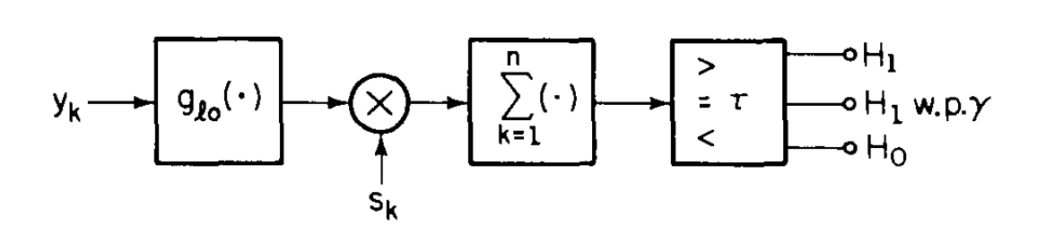
\[L(\mathbf{y}) = \prod_{k=1}^n L_k(y_k),\quad\text{where } \underbrace{L_k(y_k) = \frac{p_{N_k}(y_k-s_{1k})}{p_{N_k}(y_k-s_{0k})}}_{\text{noise density at time }k}\]So, since comparing $L(y)$ to $\tau$ is like comparing $\log L(y)$ to $\log\tau$, the detection structure is like follows:
\[y_k \;\longrightarrow\; \boxed{\log L_k(\,\cdot\,)} \;\longrightarrow\; \boxed{\displaystyle \sum_{k=1}^{n}(\,\cdot\,)} \;\longrightarrow\; \boxed{ \begin{array}{c} > \log \tau \;\Rightarrow\; H_1 \\[4pt] = \log \tau \;\Rightarrow\; H_1 \text{ or } H_0 \\[4pt] < \log \tau \;\Rightarrow\; H_0 \end{array} }\]Coherent detection in $\text{i.i.d.}$ Gaussian noise
$N_1,N_2,\dots,N_n$ are independent are identically distributed $\mathcal{N}(0,\sigma^2)$. Assume WLOG $\mathbf{s}_0 = \mathbf{0}$ (the zero signal is zero, since if we know it we can just subtract it off). We further call $\mathbf{s}_1$ just $\mathbf{s}$.
From the example of location testing with Gaussian error (see previous or ex II.B.2 in book), $\log L_k(y_k)=s_k(y_k-s_k/2)/\sigma^2$.
\[\hat{\delta}_0(y) = \begin{cases} 1,\quad \text{if}\quad\cdot > \cdot \\ \gamma,\quad\text{if } \sum_{k=1}^ns_k(y_k-s_k/2) = \sigma^2\log\tau \\ 0,\quad \text{if}\quad\cdot > \cdot \end{cases}\]This is known as a correlation detector.
An important feature of this optimum detector for Gaussian noise is that it operates by comparing the output of a linear system to a threshold. In particular, we can write
\[\sum_{k=1}^{n} s_k y_k \;=\; \sum_{k=-\infty}^{n} h_{n-k} \, y_k,\]where
\[h_k = \begin{cases} s_{n-k}, & 0 \le k \le n-1, \\ 0, & \text{otherwise}. \end{cases}\]Hence, this detector can be viewed as a system that inputs the observation sequence $y_1,\dots,y_n$ to a digital linear filter and then samples the output at time $n$ for comparison to a threshold. This structure is known as a matched filter
Note: the term coherent detection is used , since these signals can be sinusoids which has a phase, and so if the phase is known then the signal is completely known (and if not, then it is non-coherent signal detection).
What if we have other noise, not Gaussian?
Coherent Detection in $\text{i.i.d.}$ Laplacian noise
This is the same problem as previous but noise $N_1,dots,N_n$ is i.i.d. Laplcian noise, i.e.
\[p_{N_k}(n_k) = \frac{\alpha}{2}e^{-\alpha\lvert n_k\rvert},\quad n_k\in\mathbb{R}\]This may be called ‘impulsive noise’ or ‘long-tailed noise’. We get a little more interesting detector structe, since we no longer get a linear likelihood ratio.
\[\log L_k(y_k) = \begin{cases} -\alpha |s_k|, & \text{if } \operatorname{sgn}(s_k)\, y_k \le 0, \\[6pt] \alpha \left| 2y_k - s_k \right|, & \text{if } 0 < \operatorname{sgn}(s_k)\, y_k < |s_k|, \\[6pt] +\alpha |s_k|, & \text{if } \operatorname{sgn}(s_k)\, y_k \ge |s_k|. \end{cases}\]Below are the two graphs of $\log L_k(y_k)$ vs, $y_k$ for $s_k>0$ and $s_k<0$.
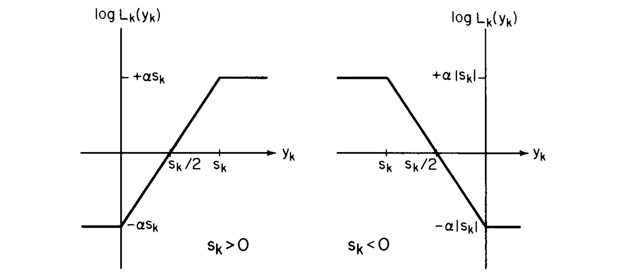
Here, we have longer-tails, so we are more likely to have higher observations to come from noise, and hence we want some way of ‘blanking’ these out as above.
This structure is known as an amplifier limiter.
Locally optimum detection of coherent signals in $\text{i.i.d.}$ noise
We consider,
\[H_0: Y_k=N_k\text{ vs. }H_1: Y_k = N_k+\theta s_k\quad\text{ for }k=1,\dots,n,\]where $\mathbf{s}$ is a known signal and $\mathbf{N}$ is a continuous random noise vector with i.i.d. components.
This is an example of a parametric signal, where $\theta$ is the amplitude / ‘signal strength parameter’ (e.g. radar problem could fit into this setup).
Given $\theta$, we have the likelihood ratio,
\[L_\theta(\mathbf{y}) = \prod_{k=1}^n\frac{p_{N_k}(y_k-\theta s_k)}{p_{N_k}(y_k)},\]where $p_{N_k}$ is the marginal density function. The locally optimum test for $H_0$ vs. $H_1$ is,
\[\tilde{\delta}_{l_0}(y) = \begin{cases} 1, & \cdot>\cdot \\ \gamma, & \text{if } \left. \frac{\partial}{\partial \theta} L_\theta(y) \right|_{\theta=0} = \displaystyle \sum_{k=1}^{n} s_k\, g_{l_0}(y_k) = \tau \\ 0, & \cdot < \cdot \end{cases}.\]Here, the detector is (again) a correlator, although it is specifically a non-linear correlator.
The non-linearity depends on the noise distribution, and it comes from the $g_{lo}(x) = p_N’(x) / p_N(x)$, which doesn’t necessarily have to be linear.
$g_{lo}$ is known as the ‘scores function’; it determines how you ‘score’ the data. It tells you how to process the data when it comes in. From a statistics perspective, we could draw an analogy of this as being a sufficent statistic; this is the information you need to know about the data
If the noise is $\mathcal{N}(0,\sigma^2)$, then $g_{lo}(x)=x/\sigma^2$ is linear.
If the noise is Laplacian, $g_{lo}(x)\alpha\operatorname{sgn}(x)$.
Another interesting case is if the noise has Cauchy distribution (a very heavy-tailed ditribution, in fact is has variance $\infty$).
\[p_N(x) = \frac{1}{\pi(1+x^2)},\quad\text{and so }g_{lo}(x) = \frac{2x}{1+x^2},\quad x\in\mathbb{R}.\]